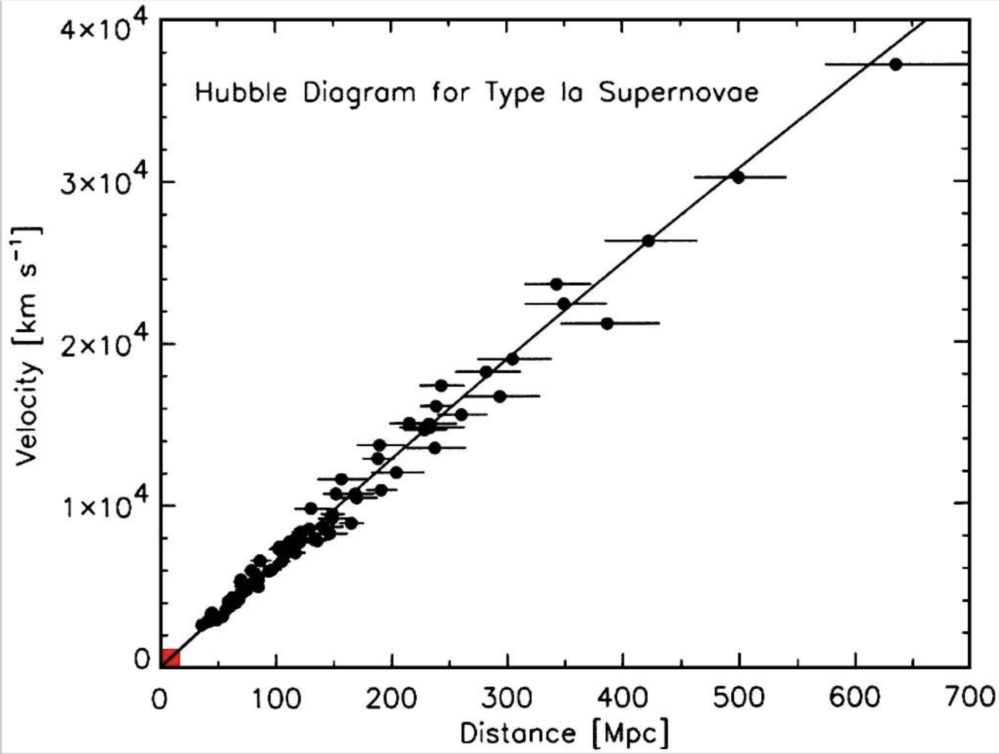
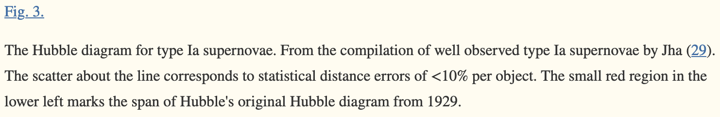
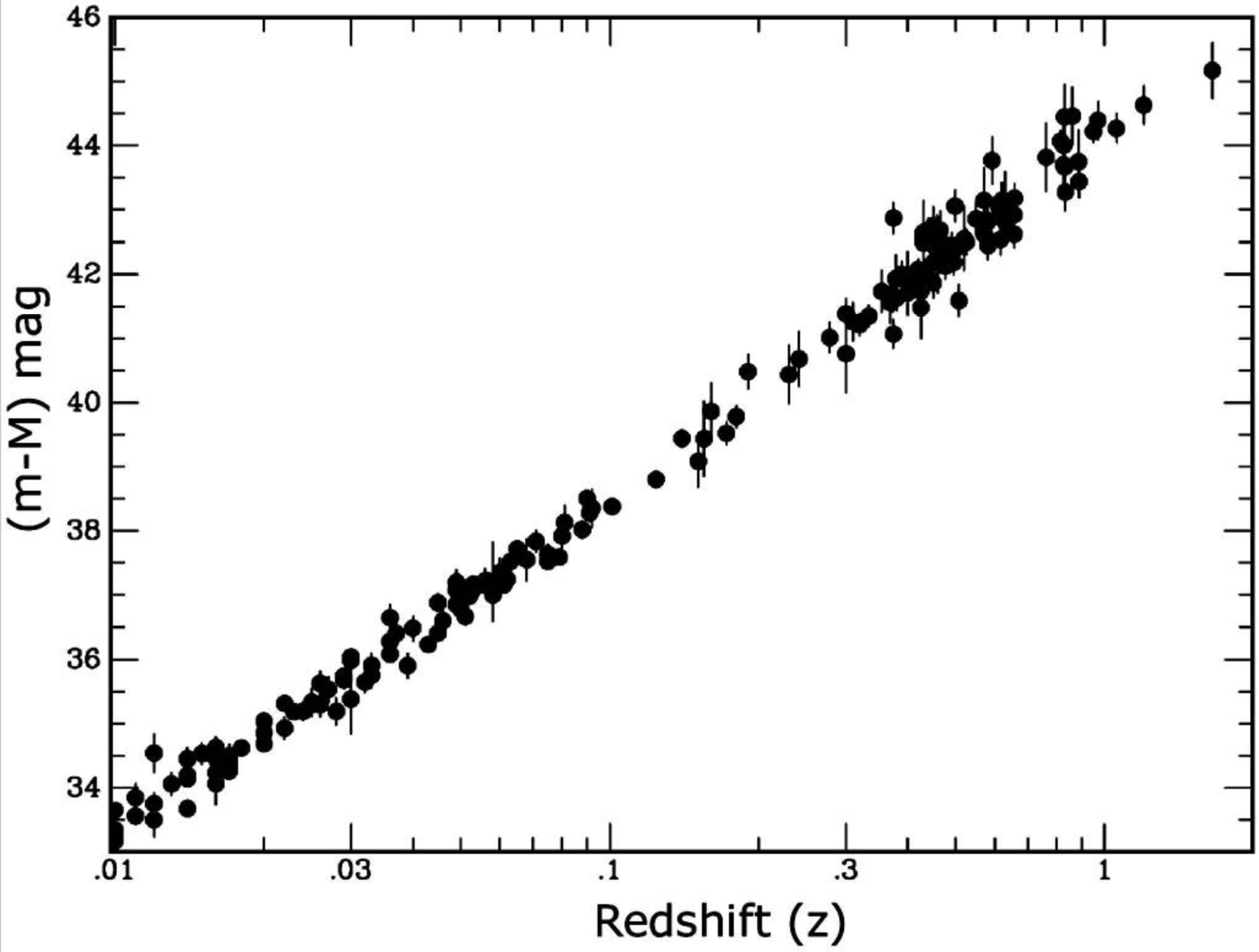
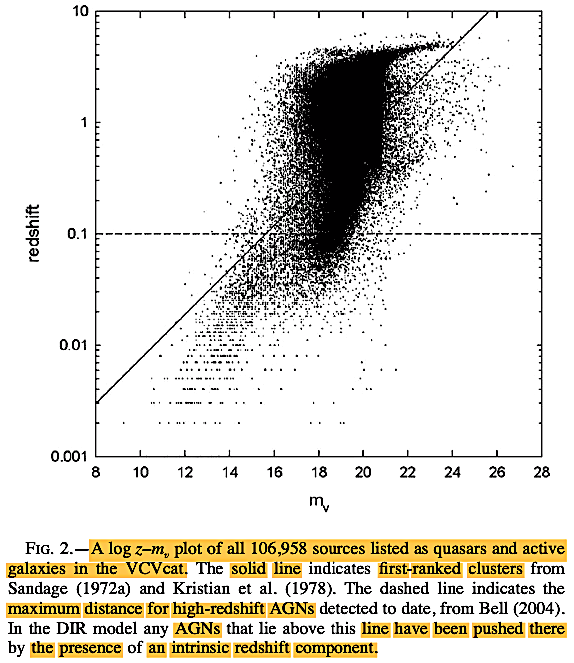
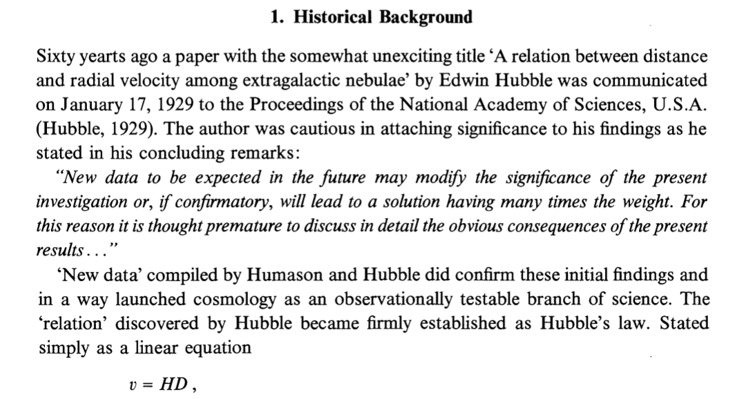
VII. Unexpected Galactic Redshifts
![]()
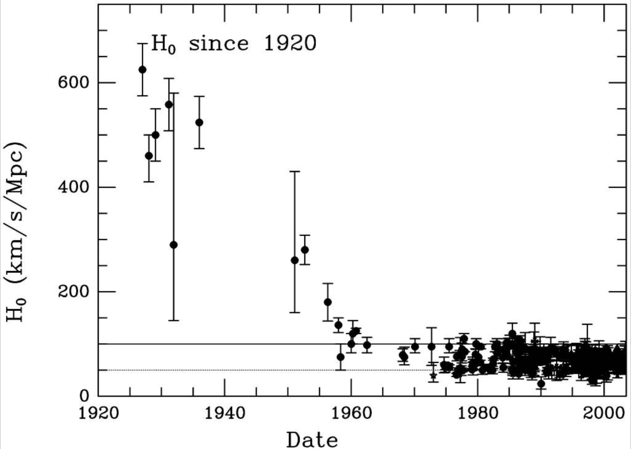
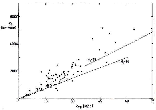
Expected Hubble distance-velocity relation
1930: H0 = 558
km s−1
Mpc−1
Intervening years: H0
= 30-100 km s−1
Mpc−1
Today, although narrowed,
we still have a range of values: H0 =
~63-75 km s−1
Mpc−1
  |
  |
    |
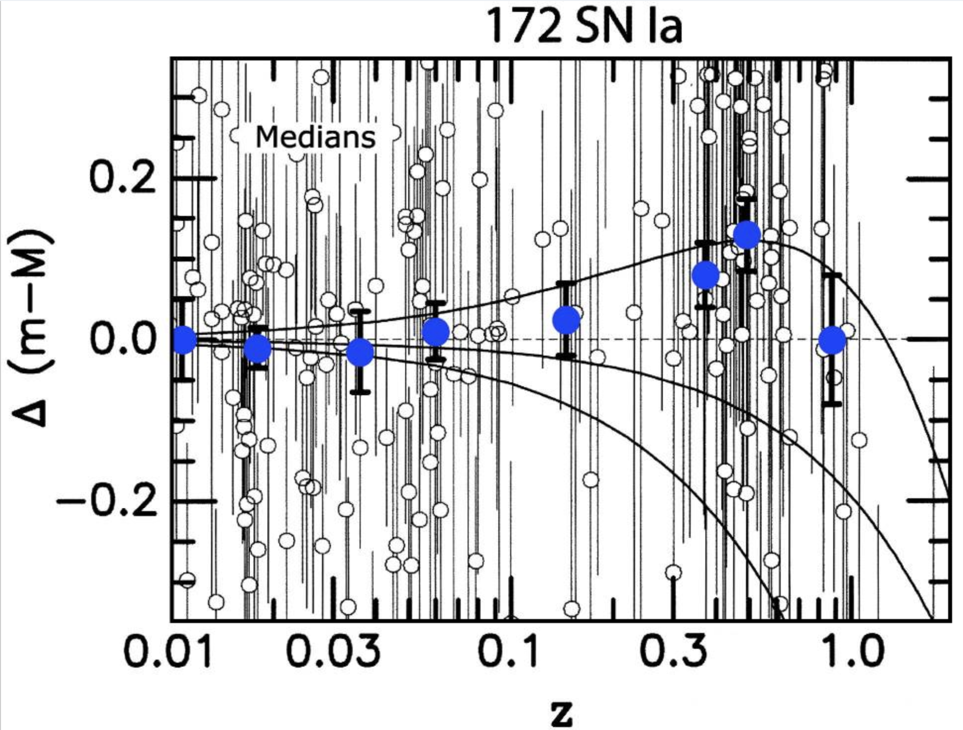  |
Above, we see
the 2004 estimates of the SN1a acceleration data compared
with various HBBC models with chosen proportions of 'dark
energy' and 'dark matter' (Kirshner, 2004; link).
Their review was in many ways far too simplistic to fully
consider the magnitude and complications of the ad hoc
free-parameter fitting required in HBBC models.
In the NASA
website of the Lambda working group, they attempted to
provide a summary of the many estimated values of the Hubble
constant H0
from a series of major studies done from 2001 to 2021. This
serves to highlight the difficulties of nailing down this
supposed constant:
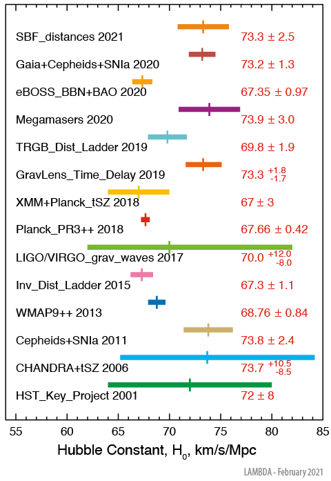
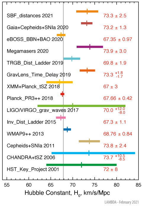
Hubble Constant (NASA / LAMBDA Archive Team; link)
PNG
(480 x 697 px) 38Kb PNG
(1024 x 1488 px) 39kb PNG
(2048 x 2975 px) 194kb
PDF
77kb (Vector Art) SVG
57kb (Vector Art) EPS
41kb (Vector Art).(https://lambda.gsfc.nasa.gov/education/graphic_history/hubb_const.cfm).
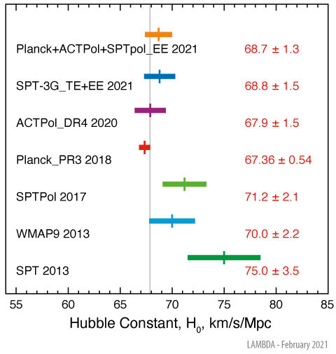
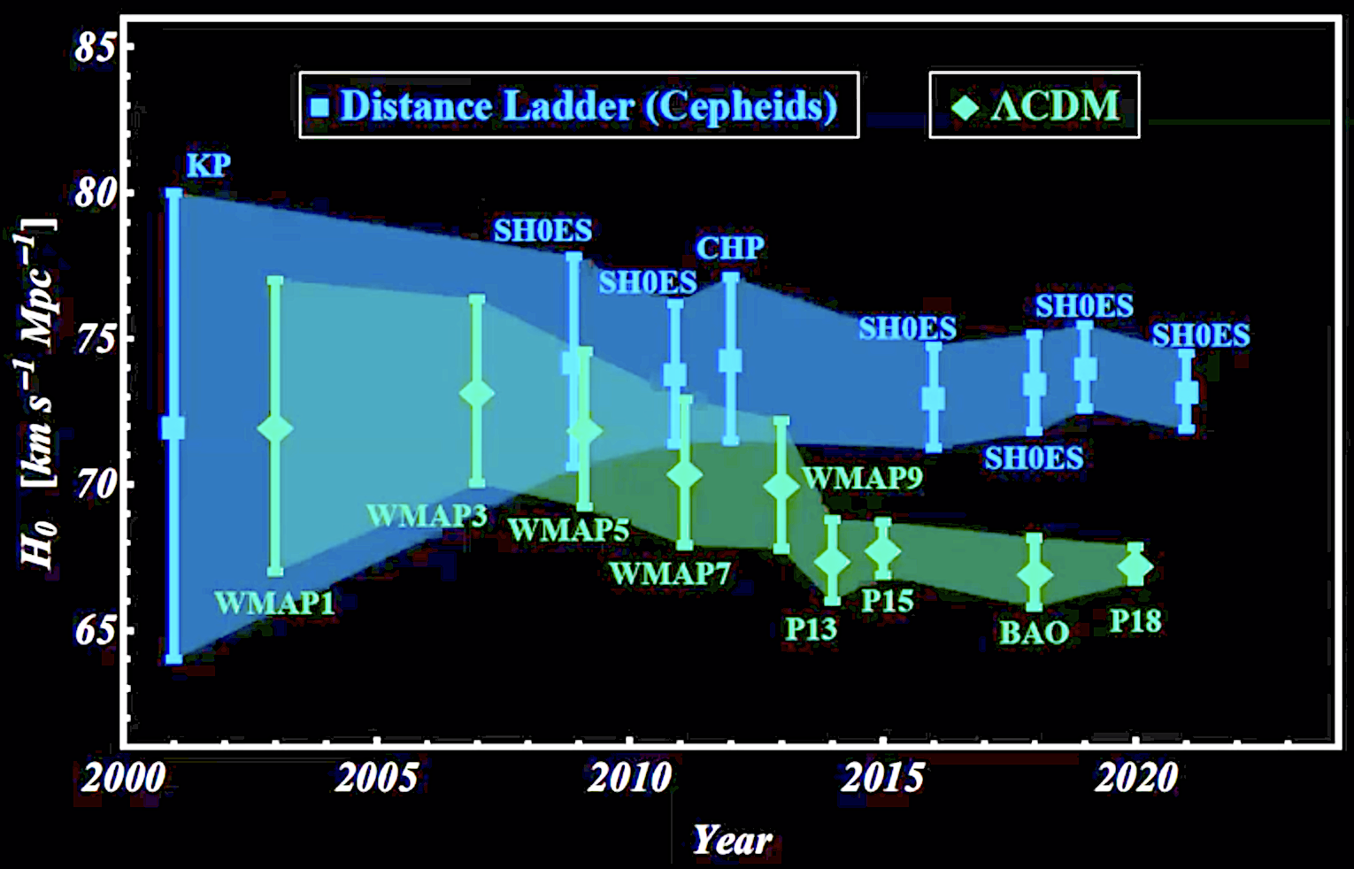
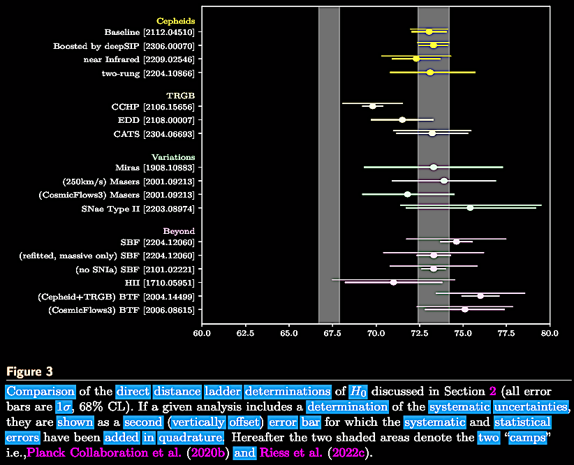
Over recent years, there has been a growing disagreement between estimating the Hubble constant, H0, using more local distance measures with (often a very few) 'standard candles' such as Cepheid variables and red giants (~72-73 or even 75 +/- 2.3, &c., km s−1 Mpc−1 ) and those estimated by supposedly early universe parameters of the CMB which are model-derived by the CDM and ΛCDM versions of the HBBC (~67-69 km s−1 Mpc−1 ; see citations on the disconnect controversy link, link, and link). Despite the above claims of approaching resolution between 'standard candle' and model-dependent estimates of H0, as of 2022, the discrepancies are gaping, as indicated in a selection of recent papers.
- For a few
examples, de Jaeger et al. (March 2022) in their
attempts to resolve the "Hubble tension" tried the
following: using
"13 SNe~II with geometric, Cepheid, or tip of
the red giant branch (TRGB) host-galaxy distance measurements"
derived H0
= 75.4 +3.8/−
3.7 km s−1
Mpc−1
(statistical errors only), which they claimed was "
consistent with the local measurement but
in disagreement by ~2σ from +ΛCDM value." Also, de
Jaeger et al. using Cepheid variables only
with a sample size of N = 7, arrived at H0
= 77.6 + 5.2/−
3.7 km s−1
Mpc−1
, and when using only red giants (TRGB) with a
sample size of N = 5, found H0
= 73.1 + 5.7/−
5.3 km s−1
Mpc−1
.
They further claim they did not find that the SNe~1e
or the Cepheids were the source of the "H0
tension" while admitting that their "conclusions rest
upon a modest calibrator sample," and urge that larger
studies be done in future (
arXiv:2203.08974).
- In April 2022, Cao & Ratra (2022) claimed to use non-CMB and "model-independent determinations" with " updated Hubble parameter and baryon acoustic oscillation data, as well as other lower-redshift Type Ia supernova, Mg II reverberation-measured quasar, quasar angular size, H II starburst galaxy, and Amati-correlated gamma-ray burst data, to jointly constrain cosmological parameters in six cosmological models," to arrive at H0 = 69.7 +/− 1.2 km s−1 Mpc−1 , " the flat ΛCDM model is most favored but mild dark energy dynamics and a little spatial curvature are not ruled out" ( arXiv:2203.10825).
- In March
2022, Hu & Wang (link) reported that the "Hubble
crisis" may be relieved by having H0
change over cosmic time from the
early universe to the present epoch
(arXiv:2203.13037).
Anand
et al. in March of 2022 instruct the reader to
"worry no more, the Hubble tension is relieved" because
they made local cosmic measurements using inferences
from sedimentary and eclipse-based data of the lunar
recession velocity to arrive at H0
= 63.01 +/−
1.79 km s−1 Mpc−1,
which they tout as the first single-step,
model-independent measure of the Hubble constant, which
also is not far from CMB and the ΛCDM model determinations, concluding that
local measurements are the source of the Hubble
tension (
arXiv:2203.16551).
- In April
2022, Liu et al. also claim a model-independent
cosmography method of directly measuring by
reconstructing distance based on cosmic chronometer and
gravitational lensing observations, as well as a
measurement of space-time curvature, while avoiding the
polynomial curve-fitting and what the polynomial
coefficients might physically mean: H0
= 72.24 +2.73/−
2.52 km s−1
Mpc−1
(arXiv:2204.07365).
When assuming a flat universe in advance, they arrive at
H0
= 70.47 +1.14/−
1.15 km s−1
Mpc−1
, between the Planck CMB and the SH0ES observations.
- In late April, the large group of Kenworthy et al. ( arXiv:2204.10866) used a 3 rung distance ladder of calibrating Type Ia supernovae using a SH0ES measurement for the host galaxies of 35 Cepheid variables at cz < 3300 km s−1 , geometrically calibrated in our Milky Way, NGC 4258, and the Large Magellanic Cloud (LMC), and arrived under various assumptions including peculiar velocities at z ~ 0.01 at a range of H0 = 71.8 to 77.0 km s−1 Mpc−1 . By combining the four best fitting selection models, they estimated H0 = 73.1 to 77.0 km s−1 Mpc−1 , which is 2σ removed from the Planck results.
- Also in April
2022, Garnavich et al. (
arXiv:2204.12060)
compared infrared surface brightness fluctuations (IR
SBF) in galaxies hosting type Ia supernovae (SNIa) to
distances estimated by SNIa light curve fitting, showing
that IR SBF estimates are different from those derived
from Cepheid variable calibrators. Using IR SBF results
from massive galaxies surveye within ~100 Mpc by Jensen
et al. (2021;
arXiv:2105.08299), Garnavich and
colleagues arrived on basis of 25 SNIa host galaxies at
H0
= 74.6 +/−
0.9(stat) +/−
2.7 (syst) km s−1
Mpc−1
,
including both statistical errors and systematic errors,
and thus consistent with supernovae distances calibrated
with Cepheids.
- In early May
2022, Renzi and Martinelli (
arXiv:2205.03396)
propose that using super massive black hole (SMBH)
shadows on galaxies as a distance anchor in the distance
ladder, in place of Cepheids for example, will be able
to constrain H0
values within
H0
≈ 10% for
current ground
based
interferometers
and within H0 ≈ 4% for
future interferometers.
- Another team in May 2022, Breuval et al (including Adam Riess; arXiv:2205.06280) added an improved calibration for the wavelength dependence of metallicity on the Cepheid Leavitt law, and cepheid brightness does depend on metallicity. Why such a calibration needs to be done of course drops a hint indirectly that other factors need to be taken into account when considering galactic redshift, not limited to be a result of space-time expansion. (More on that).
- Reviewing
developments, Blanshard et al (
arXiv:2205.05017)
in May of 2022 reviewed the tensions in the measurement
of H0
and
estimates of matter density within the ΛCDM and
some "alternative cosmological models" (CDMs without Λ) highlighting the
tensions. They say that data on cosmic chronometers
allow derivation of an accurate value at H0
= 67.4 +/−
1.34 km s−1
Mpc−1
.
Nevertheless, they came to the conclusion that
the ΛCDM model is "alive
and well"
but has "an unknown bias in the Cepheids distance
calibration" and celebrate a remarkable agreement for
the model, statistically better than the previously
proposed extensions with H0
~ 73.
- In late May
2022, Chen et al (
arXiv:2205.11278)
arguing that gravitational waves (GW) are another way to
probe the Universe's expansion history, and adopt the
assumption that binary black hole (BBH) coalescent
events involve black holes detected by LIGO-Virgo-KAGRA
(LVK) collaboration are primordial in origin, using 43
BBH events from the third LVK GW transient catalog
(GWTC-3). Using three PBH mass models and some Bayesian
population analysis, they concluded that the constraints
on the ΛCDM model
cosmological parameters "are rather
weak and in agreement with current
results." When combining in
a measurement from GW170817 (a LIGO / Virgo GW signal of
merging neutron stars detected in 2017 in NGC 4993),
they were able to claim constraint of H0
between
69 +19/−
8
km s−1
Mpc−1
and 70 +26/−
8
km s−1
Mpc−1
,
comparable
with results
from
phenomonological
models of
astrophysical
mass models of
BH
coalescence.
- In mid May 2022, Schiavonne et al ( arXiv:2205.07033), in examining a collection of 1048 Type Ia Supernovae (SNe Ia) in the Pantheon sample database with a redshift between 0 < z < 2.26, looked to see if the H0 tension may be found among SNe Ia data using binned statistical analysis with the MCMC method for each bin, considering the ΛCDM and the w0waCDM cosmological models. They observed that H0 evolves with redshift using a fitted function, H0(z) = ~H0(1 + z)− α where ~H0 and α are two fitting parameters. Extrapolating with ~H0 back to the redshift of the last scattering estimated to be about z = 1100, where they obtain values of consistent with 1σ of the Planck CMB estimates of H0. So much for heavily model-dependent parameter fitting. However, they do discuss modified gravity models to explain the redshift varying Hubble constant, and make inferences about the postulated involvement of a scalar field potential.
Since
JWST. Since becoming fully operational in July of
2022, JWST has not resolved the questions. Just within the
arXiv database, a non-quote restricted query for 'measuring
the Hubble constant' continues to illustrate the ongoing
tensions within and beyond the >CDM paradigm for
determining H0
(1,927 results by 30 May 2024: arXiv
query; 1,920 results without 'the': arXiv query). In the more
restricted case of the quote-restricted phrase "Hubble
tension" query we have 612 results (30 May 2024: arXiv
query), whereas for the non-quote-restricted
phrase 'Hubble constant' we have 1,386 results (30 May
2024: arXiv
query). There is a large burgeoning of attempts to
resolve this tension.
Questions: Is the Hubble
tension caused by artifacts of instrumentation in
different data cohorts? Or is there a paradigmatic
reason why such a tension exists? On 28 May 2024,
physicist / physics (sometimes cosmology) popular
commentator, Sabine Hossenfelder on her YouTube channel
suggested that "A huge cosmology problem just might have
disappeared" (videolink)
citing the November of 2023 paper, which we discuss
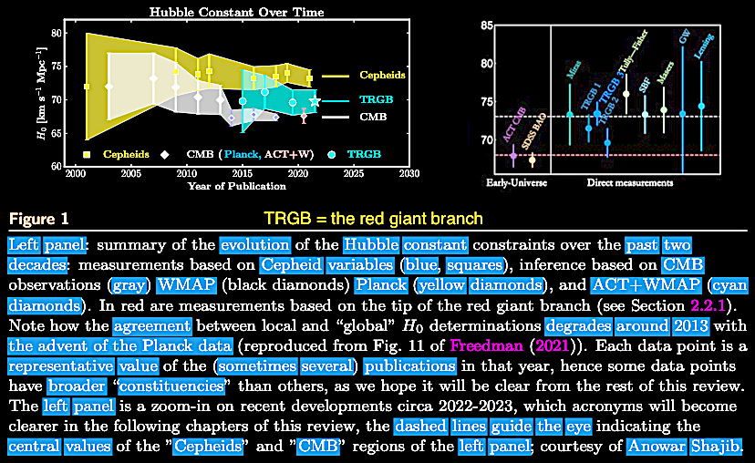
further by Freedman, W. L. & Madore, B. F. (2023).
Progress in direct measurements of the Hubble constant.
Journal of Cosmology and Astroparticle Physics (JCAP)
2023, 1-35. JCAP11(2023)050. https://iopscience.iop.org/article/10.1088/1475-7516/2023/11/050/pdf.
https://doi.org/10.1088/1475-7516/11/050.
Hossenfelder frames the issues succinctly by noting that
the Hubble tension is caused by one (any) of the
following:
- 1. Measurement error—in either the
direct redshift measurements using supernovae,
Cepheids, red giants, &c. distance ladder or the
indirect CMB redshift measurements to determine H0.
- 2. Data analysis—how the measurement
data of these competing data sets are analyzed.
- 3. Problem with the model—the
assumptions of homogeneity or isotropy of the
Universe, the distribution of mass-energy and
structure, &c.
- 4. Problem with the theory—that is,
with the field equations of general relativity,
which can vary depending on whether you are using a
'black hole' or 'bulging disk' approach. And now,
let's also add....
- 5. Perhaps the whole paradigm of the
HBBC itself needs to be re-evaluated.
In chapter
V, we discuss the Freedman & Madore (2023)
paper, the data, analyses, results, and the implications
for cosmology.
Question
for JWST: Has the James Webb Space Telescope (JWST),
which became operational in July of 2022, helped this
'tense' situation any? According to a report from November
of 2022, Yuan et al. [including 'dark energy' Nobel
laureate Adam Riess] (2022. A first look at Cepheids in Type
Ia supernova host with JWST. ApJ Letters 940,
L17. https://doi.org/10.3847/2041-8213/ac9b27),
they found that although not fully optimized for Cepheid
observation, with JWST's higher sensitivity in the near-IR
part of the spectrum, they were able to mitigate host
dust-dimming effects on distance estimates from Cepheid
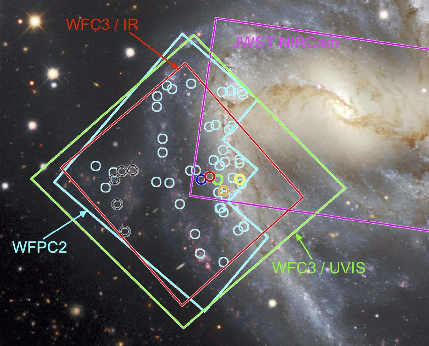
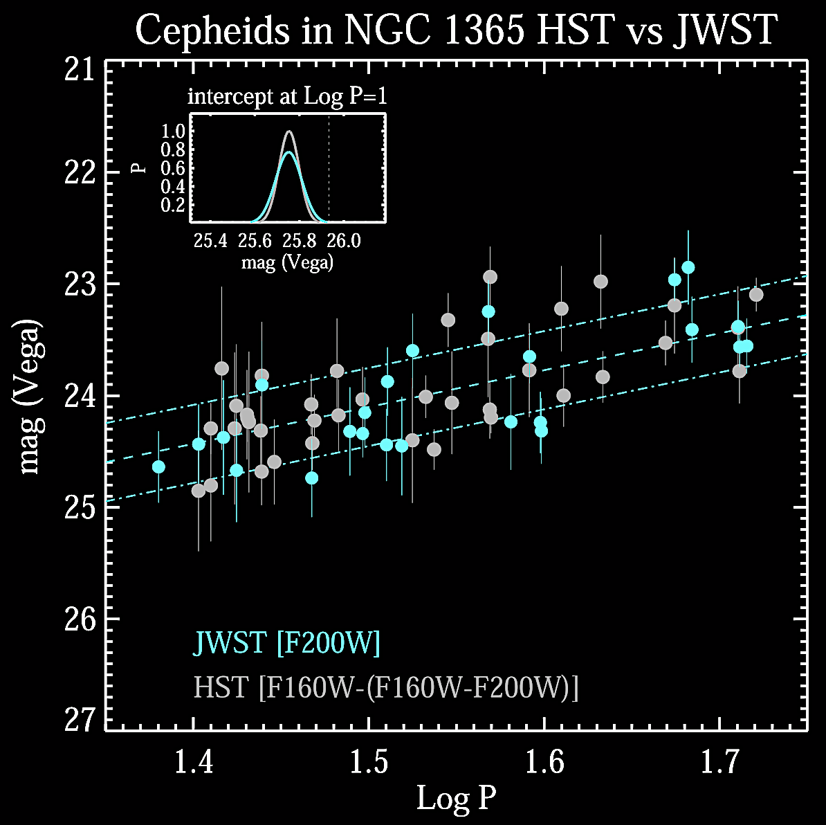
variables in NGC 1365 the host galaxy for distance
calibration of SNIa 2012fr for the Hubble constant (H0).
Using a standard star, they did photometry on 31
previously-assayed Cepheids with JWST spanning the period
(P) interval from 1.15 < log P < 1.75
including 24 Cepheids with longer P range of 1.35 < log P
< 1.75. The period-luminosity (P-L) relations of this
cohort was compared to the HST photometry results from 49
Cepheids in the full period range as well as 38 in the
longer-period interval. HST and JWST results respectively
show good agreement on P-L relations with intercepts (at log
P = 1) of magnitudes of 25.74 +/- 0.04 and 25.72 +/-
0.05. The HST-JWST Cepheid photometric consistency shows
that there's no HST-'biased-bright' error at the ~0.2
magnitude level which was suggested as a resolution to the
'Hubble tension.' See Yuan et al.'s
Figures 1 and 3 below.


Answer: No. The 'Hubble
tension' is left unresolved because it is not an
artifact of method or instrumentation, but a real
feature of the data sets, which again suggests the need
for a paradigmatic shift in cosmological theory. The
data collected from the world's next generation space
observatory, the JWST, is helping in that
direction.
Back in 2021, Di Valentino et
al. (with an author line including 'dark energy'
Nobel Laureate Adam Riess and grand master astronomer
Joseph Silk) published a 110 page monograph reviewing
>1000 peer-reviewed papers with a title parroting
Edwin Hubble's famous 1936 book title, "In the realm of
the Hubble tension—a review of solutions" in Class.
Quantum Grav. 38, 153001 (https://doi.org/10.1088/1361-6382/ac086d).
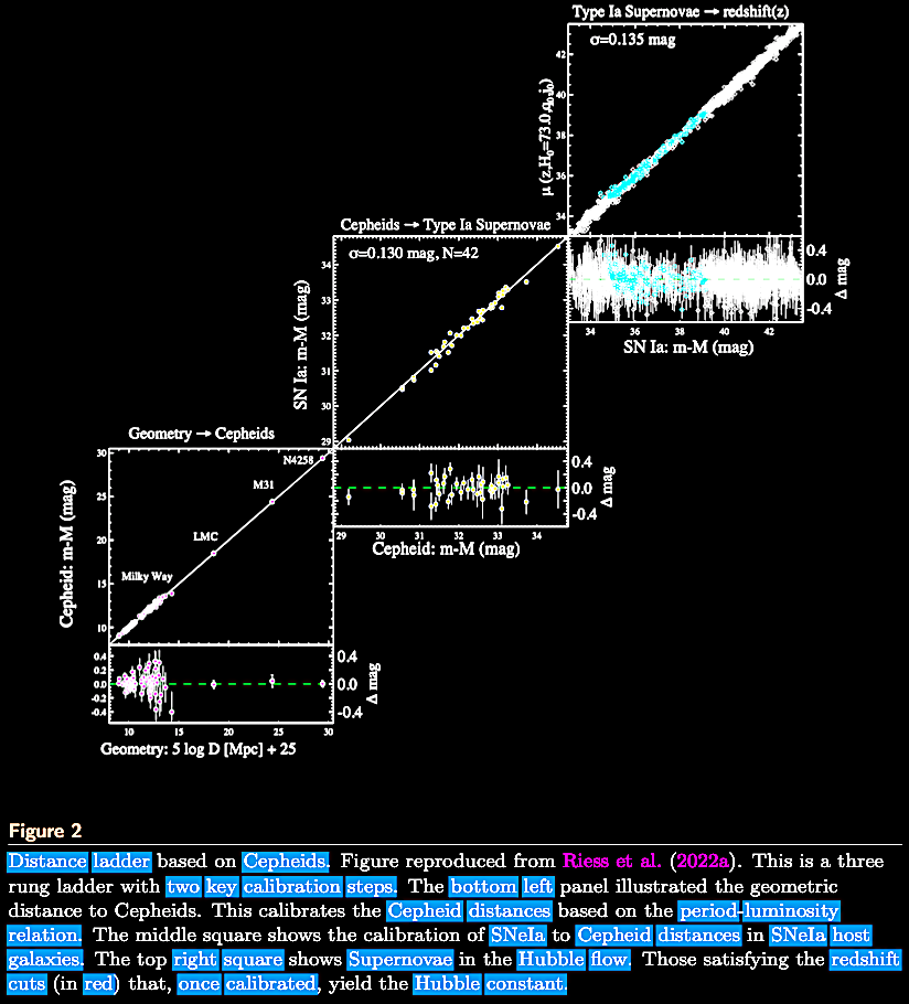
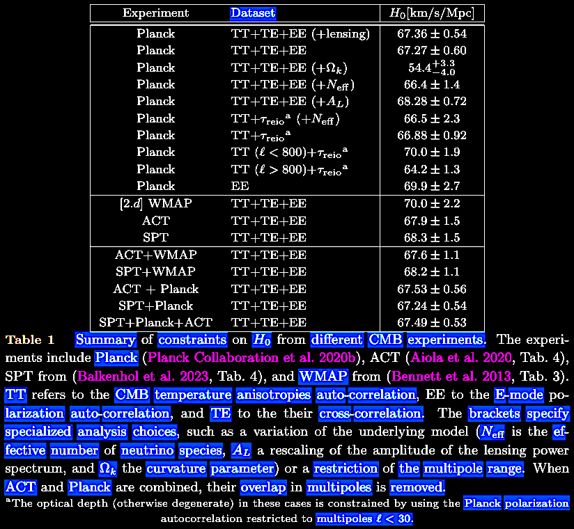
For their comparison standards, Di Valentino et al.
compared this multitude of papers to the Planck 2018 cosmic
microwave background power spectrum data with baryonic
acoustic oscillations (already loaded with adjustable ΛCDM
parameters and yielding an H0
value centered on 67.36 +/- 0.54 km s−1 Mpc−1,
according to Hart & Chluba, 2019) and
the combined Pantheon SN1e
and latest R20 data from the SH0ES Team Riess et al.
(2021, Astrophys. J. 908, L6) with an
extrapolation of the Hubble constant, H0
= 73.2 +/- 1.3 km s−1 Mpc−1 at the 68%
confidence level (CL). Like the Planck 2018 data, the SH0ES data set is itself heavily
parametrized as indicated in the mere meaning of the acronym
itself, "Supernova, H0,
for the Equation of State of Dark Energy"
(ESA press
release on the 2001-2021 SN data). Excerpted from the
many figures of the H0
values in studies cited in the monograph, one can see the
vast degree of parameter-fitting or epicycles-upon-epicycles
inserted to try to resolve this supposed constant considered
a holy grail of modern cosmology. Even with all of the
multitude of attempts to adjust parameters or create
epicycles, create complex new models, some appealing to
unknown physics, there still is a 4
σ discrepancy between these two
standards, or euphemistically we can call it a mere
'tension':
In the excerpted whisker
plots from select figures (di Valentino et al. 2021):
The vertical pink band equates with the H0 value reported by
the Planck 2018 team "within a ΛCDM scenario," while the
vertical cyan band equates with the 68% CL estimation of the
value based the SH0ES R20 data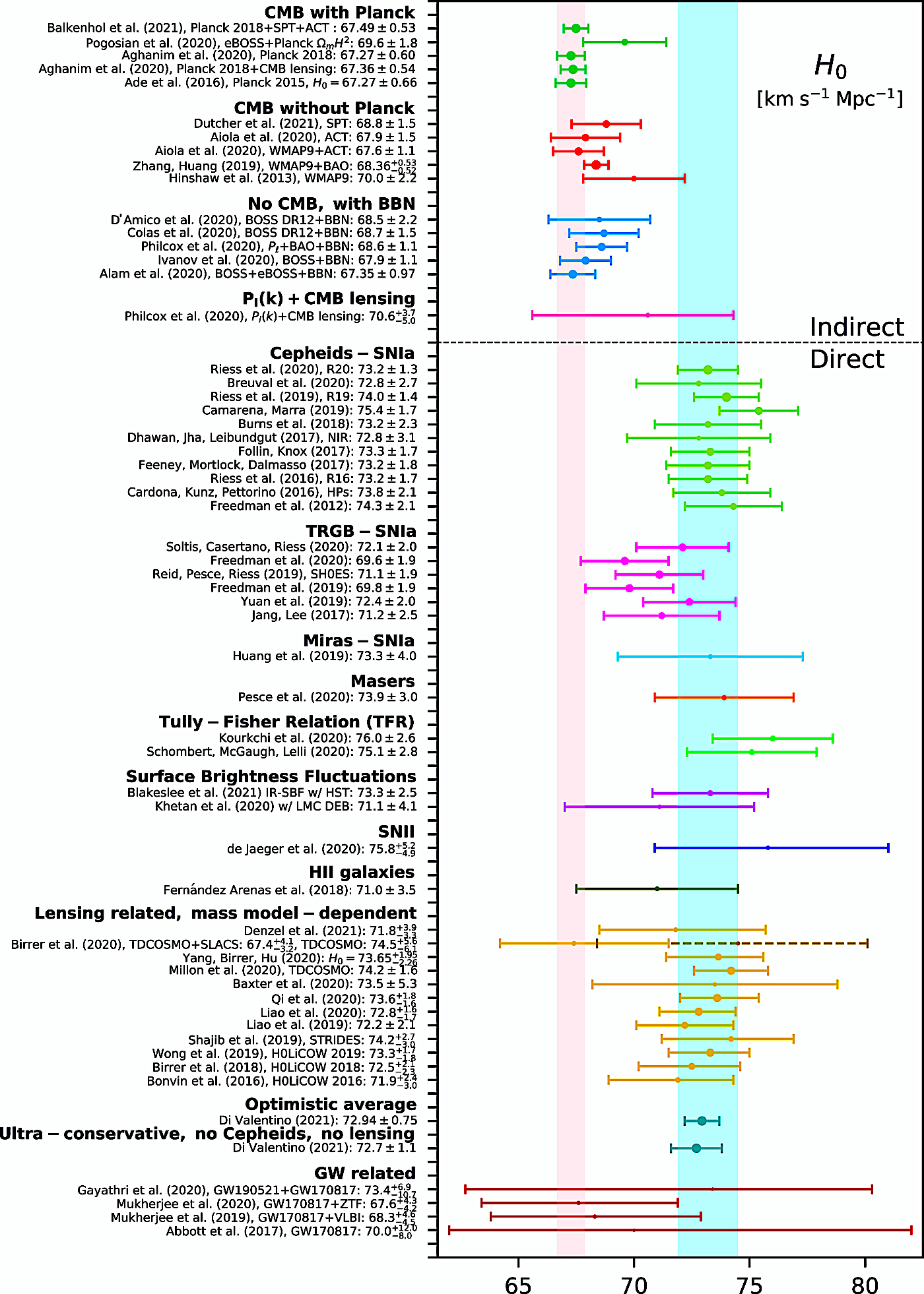
Fig. 1 (di Valentinto et al. 2021).
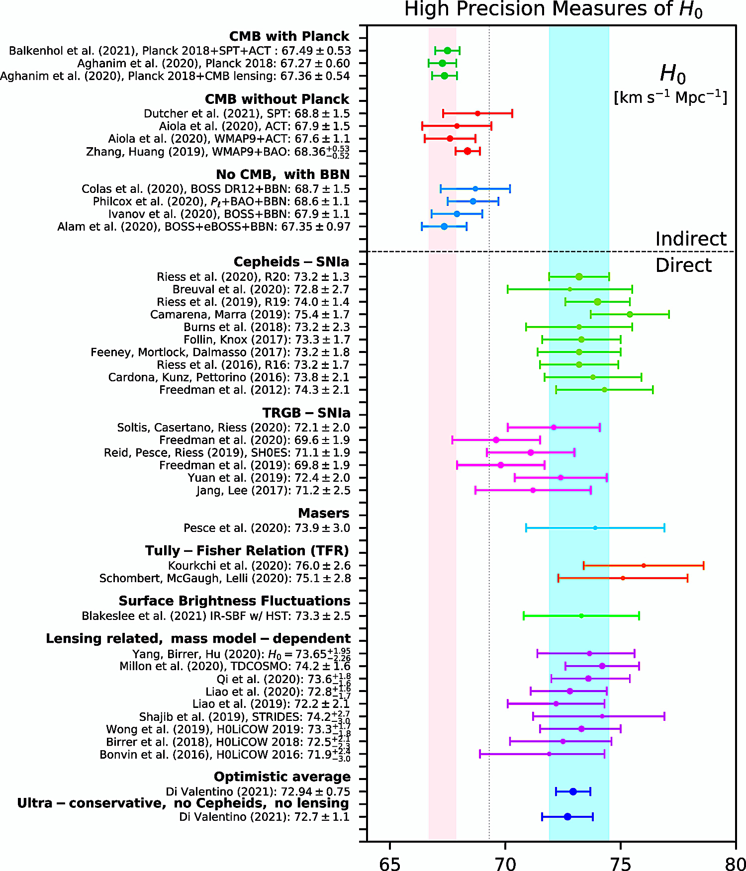
Fig. 2 (di Valentinto et al.
2021).
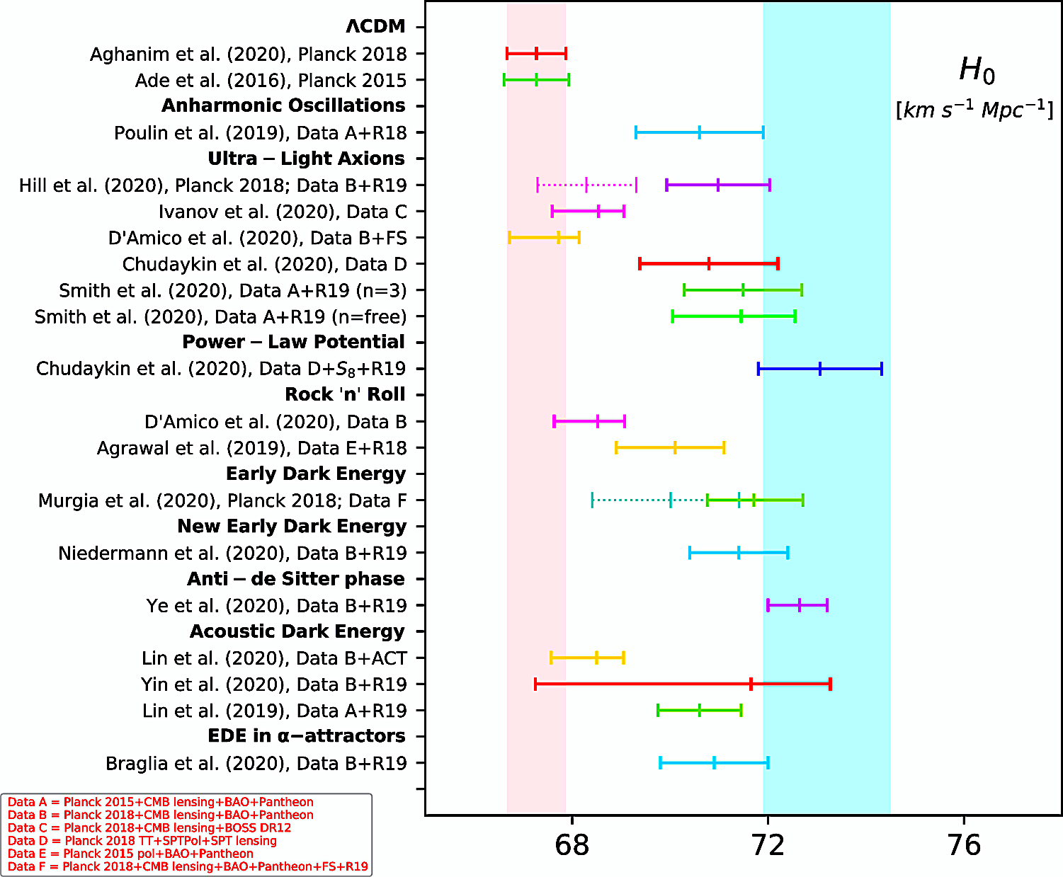
Fig. 4 (di Valentinto et al. 2021).
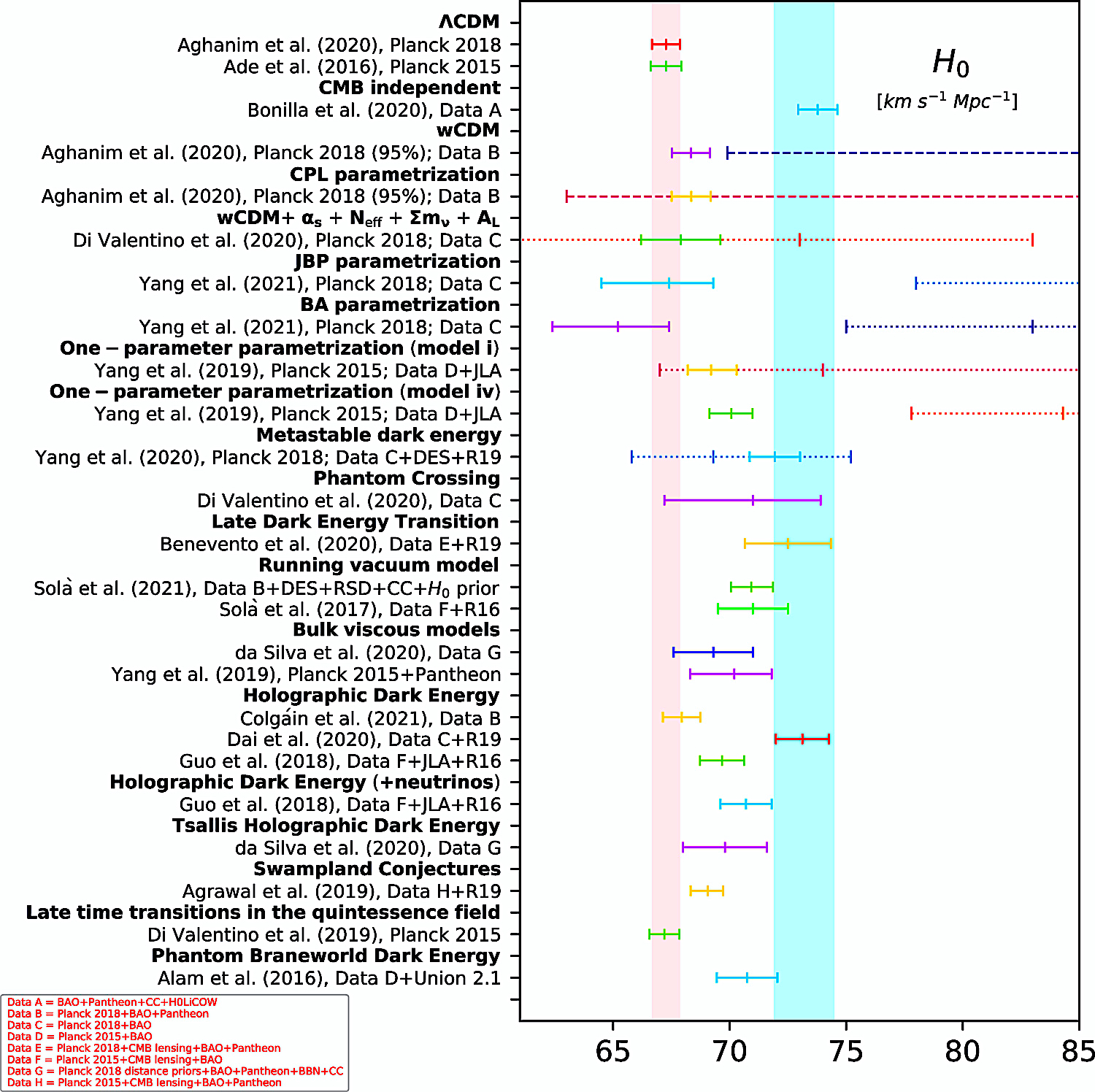
Fig. 6 (di Valentinto et al. 2021).
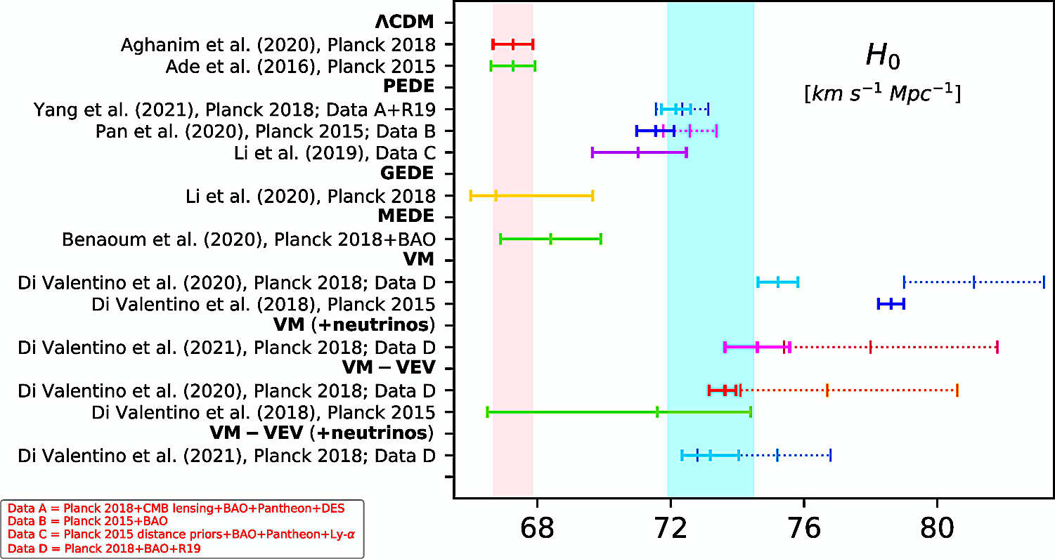
Fig. 8 (di Valentinto et al. 2021).
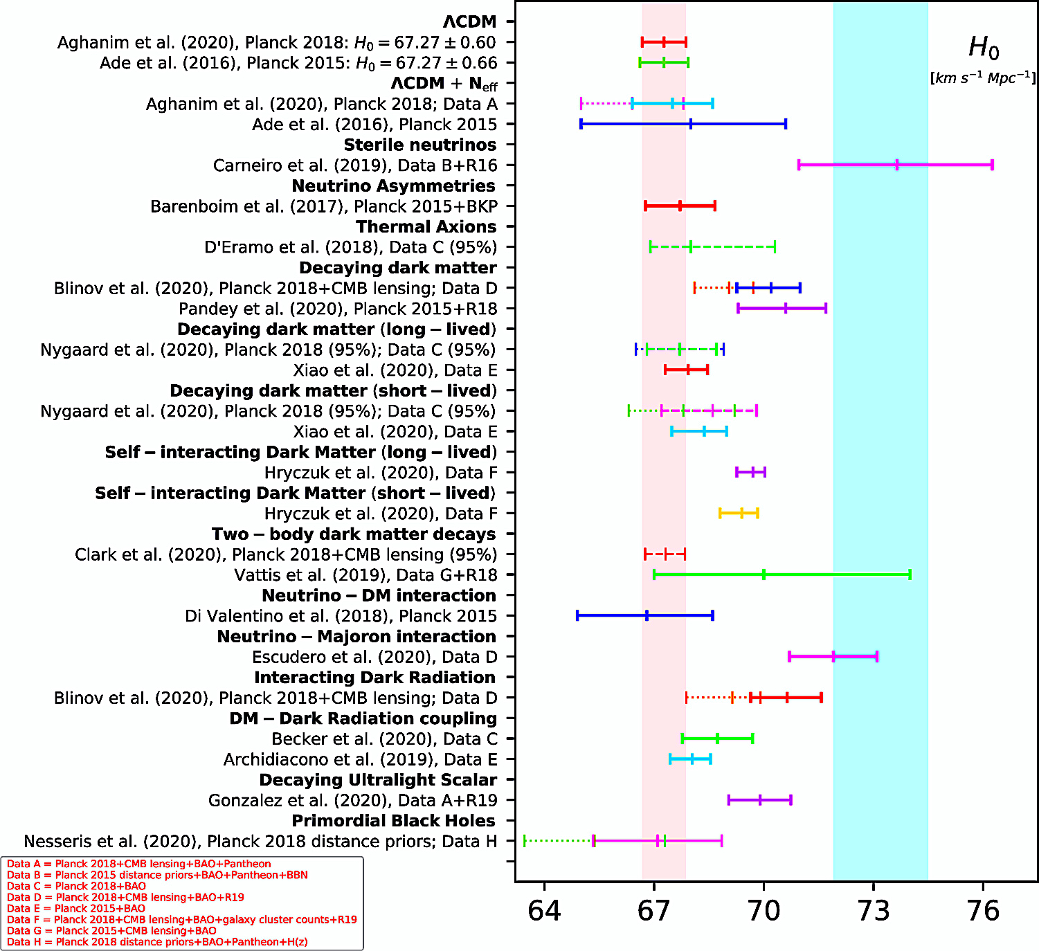
Fig. 10 (di Valentinto et al. 2021).
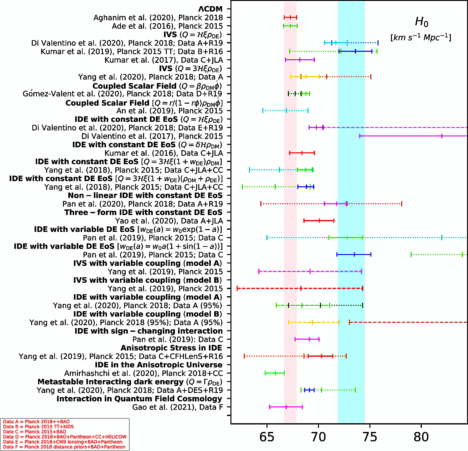
Fig. 12 (di Valentinto et al. 2021).
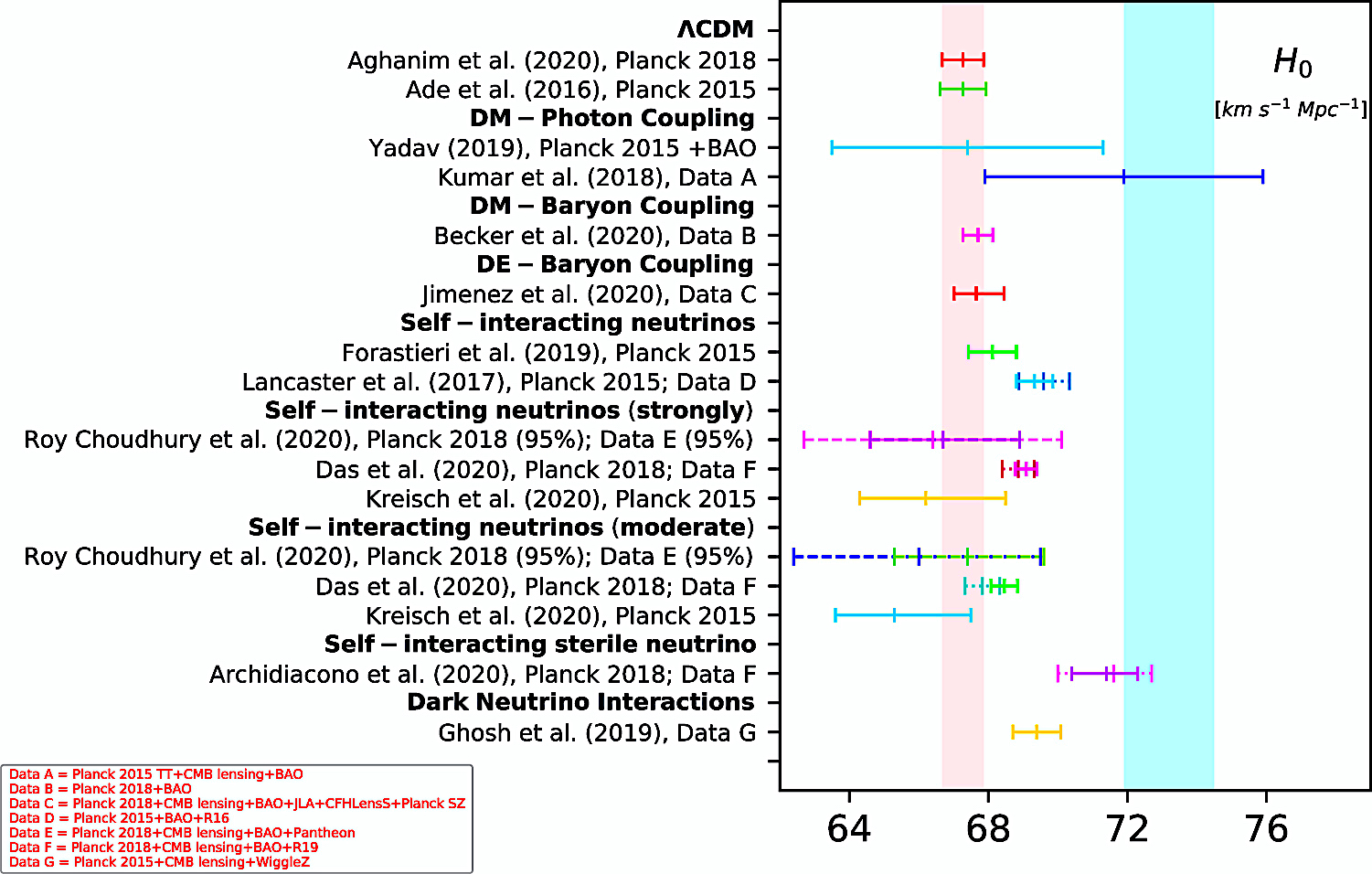
Fig. 14 (di Valentinto et al. 2021).
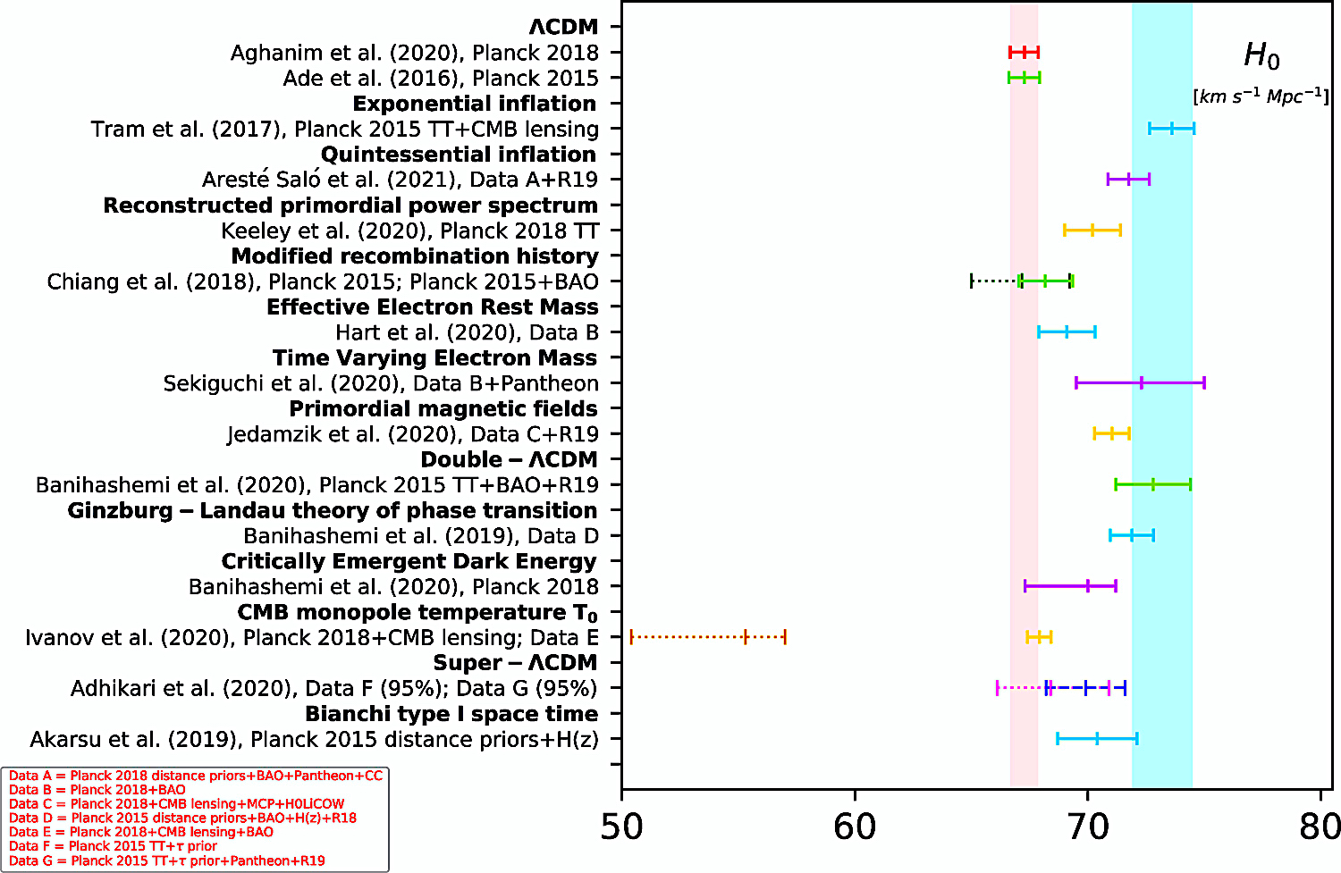
Fig. 16 (di Valentinto et al. 2021).
In
the spring of 2021, in a blog
entitled, "What is the Hubble tension, really? A
SH0ES-centric view of the problem," fellow at the Kavli
Institute of Cosmology (University of Cambridge), Sunny
Vagnozzi posted a humorous "10 commandments for Hubble
hunters" satirizing the parameter-fitting required for those
seeking to resolve the Hubble "tension." Here is the
original version, before he softened and euphemized the "4th
commandment" for a visiting lecture:
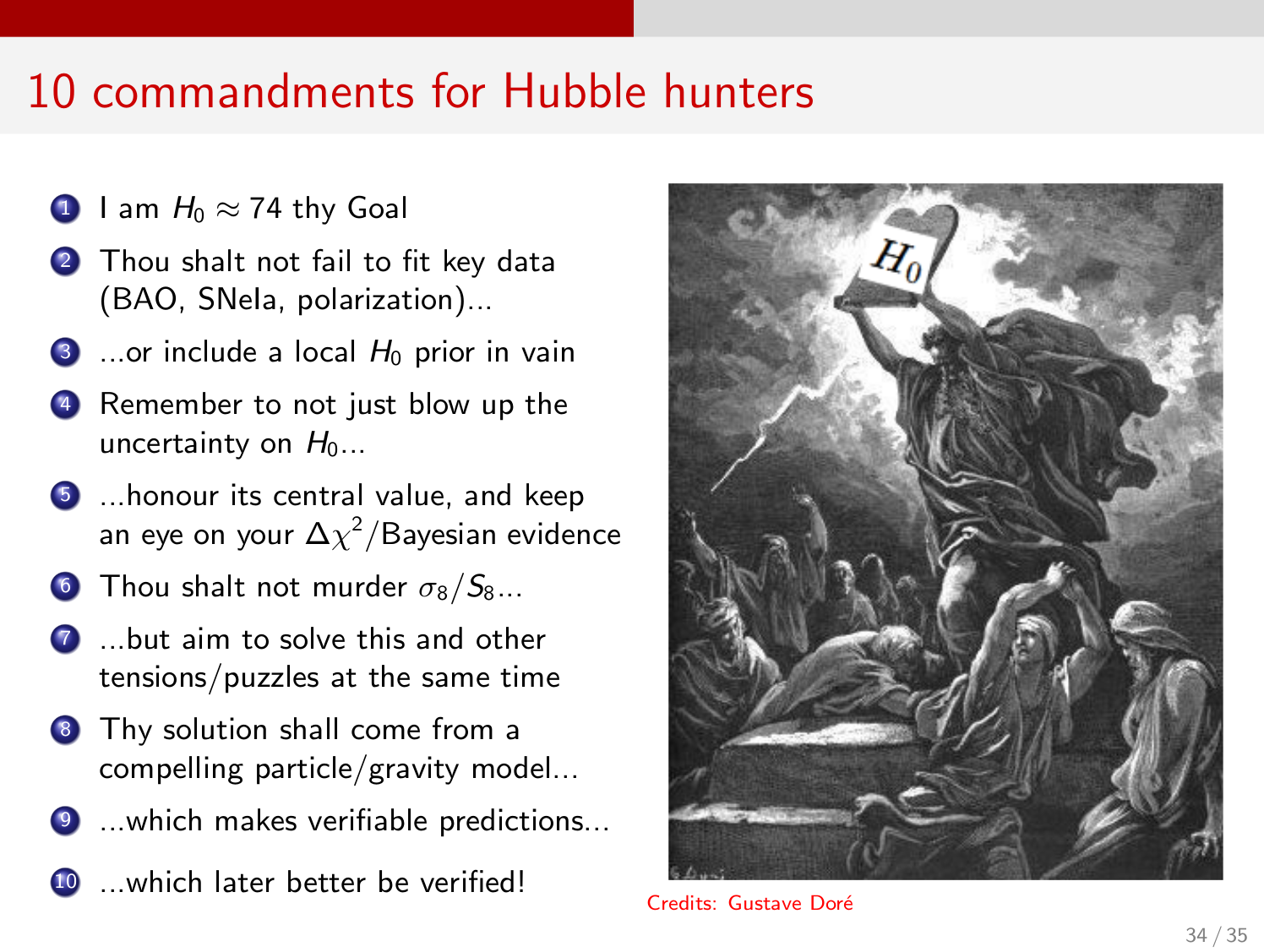
(https://www.sunnyvagnozzi.com/blog/what-is-the-hubble-tension-really).
What's
with the Hubble Constant determination Indeterminacy? What
is going on with the notorious difficulty of nailing down a
consistent, across the galactic constituent population and
across cosmic time value of H0?
Is it because H0?
varies over cosmological time?
Or is it because too narrow a
sample of 'standard candle'
bodies and the heavily
cosmological model-dependent
CMB-based calculations of H0.
What are they missing in the
cosmological data?
This
following diagram from Risaliti & Luzzo (2019;
DOI:10.1038/s41550-018-0657-z) further
illustrates the actual diversity of redshift / estimated
distance modulus with error bars in the data (including
~1600 quasars marked in yellow just with 1σ
uncertainties,
or the new
[blue-starred
marked]
quasars with z
> 3 from
the JLA
survey),
all illustrating much more redshift-diverse populations of
extragalactic objects. When set distance ladder 'standard
candle' are not the only objects included, then it becomes
obvious that the H0
relation values are not nearly so tightly
constrained as the HBBC model suggests, let alone the
highly-parameter-fitted CDM versions.
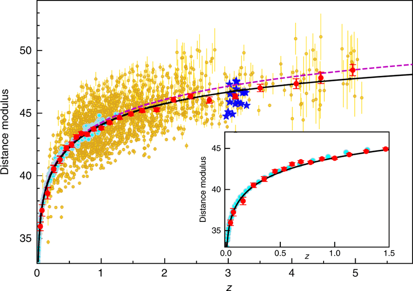
Figure legend
Figure legend (link).
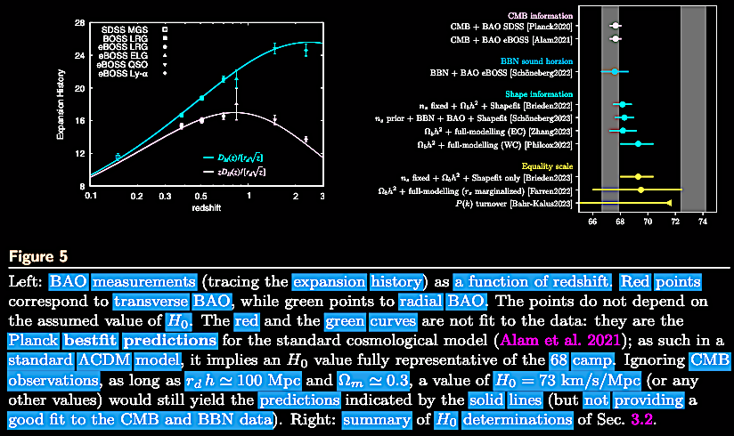
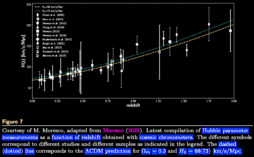
On 22 November 2023, Licia Verde, Nils Schöneberg, & Héctor Gil-Marín released a review paper on the status and meaning of the 'Hubble tension' and attempts to measure and account for it in the quest for a precision cosmology: Verde et al. 2023. A tale of many H0. https://arxiv.org/abs/2311.13305; https://doi.org/10.48550/arXiv.2311.13305. The authors point out that there are two values around with the measurements cluster: (a) the model-independent determinations from nearby galaxies with standard candles like Cepheid variables and SNIa distance ladder data of H0 = ~68 km s–1 Mpc–1 and (b) the ΛCDM model-dependent determination of H0 = ~73 km s–1 Mpc–1 based on the CMB (for a discussion of the CMB and its interpretation in cosmology, see the yet-to-be-published Chapter IV. The Cosmic Microwave Background (CMB) radiation: From Where and Whence? "As far as the eye can see?"). They suggest that there are three ways to resolve the 'tension' none of which bring consensus to the research community:
- The first is to search for systematic errors of interpretation, i.e., the systematics of the distance ladder. If those are missing, then the ΛCDM model needs modification and there are only two ways to 'fix' it:
- (i) By altering the
physics of the early time (z ≳ 1100) and "thus
the early time normalization" of the ΛCDM or
- (ii) By making "a
global modification" of the model, including questioning
the model’s basic assumptions such as the homogeneity of
the Universe, the isotropy of the Universe, and the
gravitational model of the cosmology.
 |
 |
 |
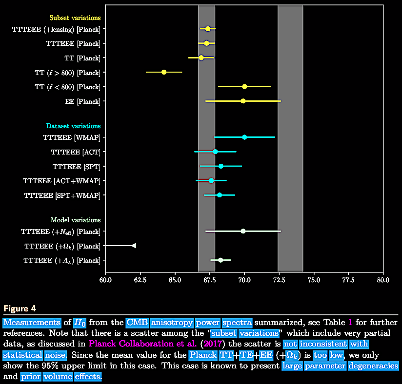 TT = temperature power..., TE = temperature-polarization cross..., & EE = polarisation power spectra, respectively. |
 BAO = baryonic acoustic oscillation. |
 |
 |
 |
Redshift anomalies: Long before the current 'Hubble tension'
Long before the ongoing 'Hubble tension' crisis in cosmology, in fact decades before a series of unexpected, non-HBBC-canonical galactic redshift anomalies began to surface, quite prior to the various 'fixes' of added epicycles to the ΛCDM version of the HBB cosmology, suggesting that something is going on which not only does not fit the HBBC in general, but has never been directly dealt with in dominant ΛCDM hot Big Bang cosmology (HBBC). We will be returning in several chapters (VIII, IX, and X, as well as possible remote JWST-discovered redshift associations in chapter V) to the subject of anomalous redshifts.
Unexpected redshifts: The complicated nature of galactic redshifts. The early start of the real problem arose when the proponents of the HBBC paradigm narrowed their focus and research to simply trying to determine and then refine "the value H0" by selected from the diversity of object-specific redshifts or z-values in any given cluster or supercluster of galaxies, rather than examining all the redshifts in any clusters and superclusters under survey to see if there are perchance any issues affecting the H0 redshift relation.
In the mid-1960s, a series of discussions stirred up by CSSC-associated cosmologists questioned whether the QSOs and their redshifts fit well into the distance-luminosity H0 models. In a pitched 'battle' between: Hoyle, F. & Burbidge, G. R. 1966. Nature 210, 1846; Hoyle. F. & Burbidge, G. R. 1966. ApJ 144, 634; and Hoyle, F., Burbidge, G. & Sargent, W. 1966. On the nature of the Quasi-stellar Sources. Nature 209, 751. https://doi.org/10.1038/209751a0, and their Big Bang interlocutors, Longair, M. 1966. Evidence on the evolutionary character of the Universe derived from recent redshift measurements. Nature 211, 949. https://doi.org/10.1038/211949a0; Sciama, D. & Rees, M. 1966. Cosmological significance of the relation between red-shift and flux density for quasars. Nature 211, 1283. https://doi.org/10.1038/2111283a0; Roeder, R. O. & Mitchell, G. F. 1966. Nature 212, 166; and Bolton, J. 1966. Identification of radio galaxies and Quasi-Stellar Objects. Nature 211, 917. https://doi.org/10.1038/211917a0. In their letter to Nature, Hoyle, F. & Burbidge, G. 1966. Relation between the red-shifts of Quasi-stellar Objects and their radio magnitudes. Nature 212, 1334. https://doi.org/10.1038/2121334a0, pointed out that these critics had misrepresented them, and jumped the gun to conclude that the QSO redshifts supported an evolutionary model (short hand for Big Bang cosmology). Sciama & Rees (1966) had gone so far as to say that the QSO redshift data ruled out the steady state (CSSC) cosmologies. As with Martin Ryle's early claims in the late 1950s about an evolving cosmos based on radiosources (see chapter III), Hoyle & Burbidge (1966) pointed out that in fact their interlocutors had jumped the gun, as it were, and that their own goals had been modest, balanced, writing:
|
"While one can certainly express a personal
preference for this latter form of argument. it
is overstating the case to claim support from it
for one cosmology or another. It appears to us
that all these discussions are predicated on the
cosmological interpretation of the red-shifts of
the quasi-stellar objects, in the sense that
this interpretation is taken as axiomatic.
Conclusions following from it are accepted,
essentially whatever they may be, because a
non-cosmological interpretation [non-BB] is
taken to be out of the question. In fact,
the issue is an open one. The difficulties
of the problem, both observational and
theoretical, lie in deciding between the
cosmological and the 'local' interpretation, not
in seeing the implications of either one of them
by itself. Throughout our work on this subject,
we have been concerned to cover both sides of
the problem, rather than to concentrate on one
half. By doing so we have been able to place
limitations on the kind of model required in the
cosmological case, as well as in the local
case."
—Hoyle
& Burbidge (1966). Nature 212, 1334 [emphasis
added].
|
So below, we begin to discuss the data which show that in fact there are other causal factors which effect the observed redshifts of various kinds of galaxies and galactic objects which do not conform to the simple Hubble relation. Specific types of galaxies which do not neatly conform to the expected redshifts of the 'standard candles' even if they are apparently in comparable distances. Some of these extragalactic sources include quasars (QSOs), BL Lacertae objects (BL Lac), Seyfert galaxies, blue stellar x-ray objects, ultra-luminous infrared galaxies (ULIRGs), and other types of active galactic nuclei (AGNs) within the clusters and superclusters in which they occur. These associated objects with different redshifts indicate that some component(s) of z may not be Hubble-distance related. Some of the first phenomena we would expect to notice then, starting with canonical Hubble relation data, are
- (0) Early canonical redshifts
in the Hubble distance-redshift relation.
- (i) Unusual
scatters in the redshift-distance relationships of large
aggregates of galaxies and galactic objects.
- (ii) Excess
redshifts dependent on galaxy morphologies.
- (iii)
Unexpected divergent redshift associations and apparent
ejection phenomena.
- (iv) Unusual
redshift periodicities which won't go away.
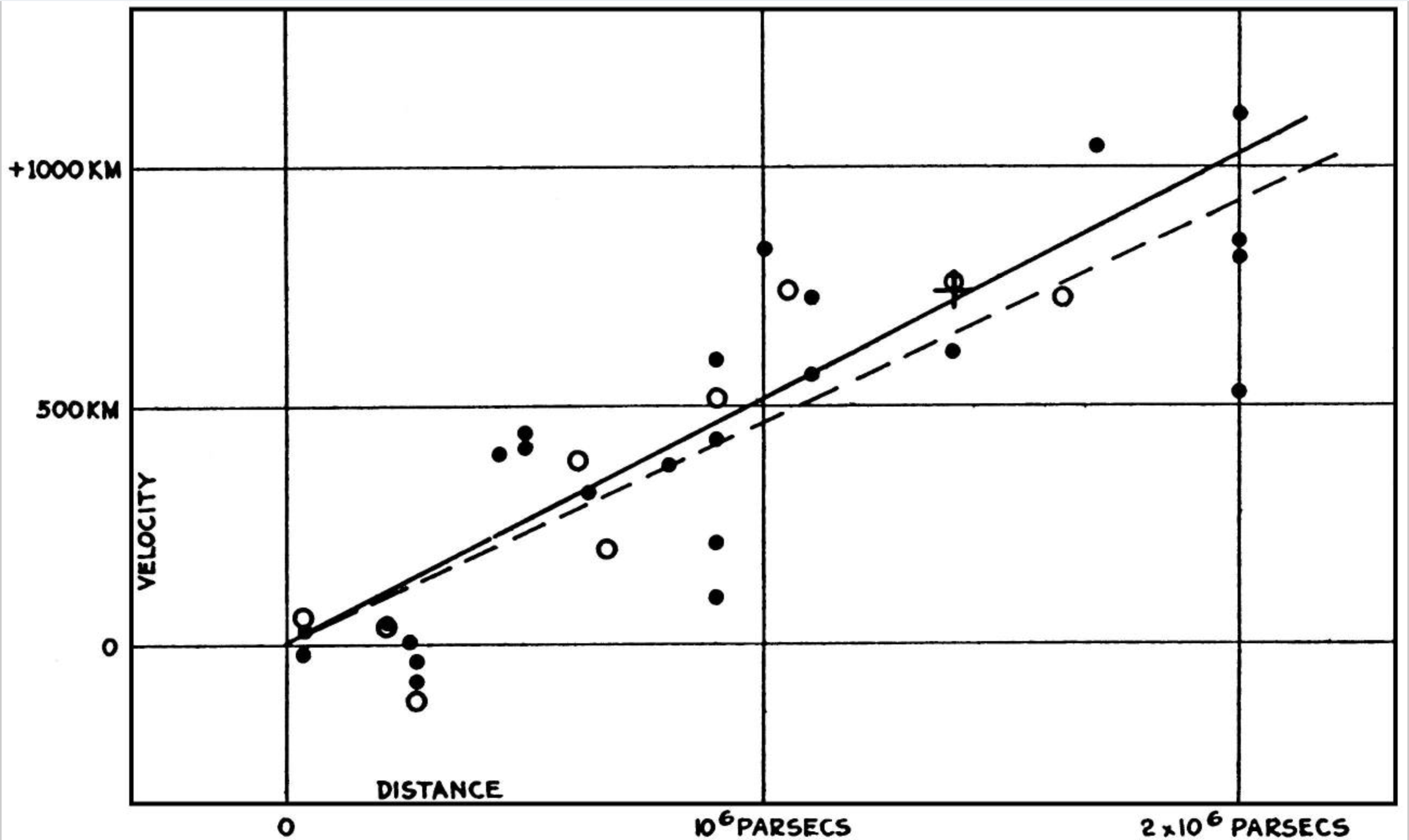
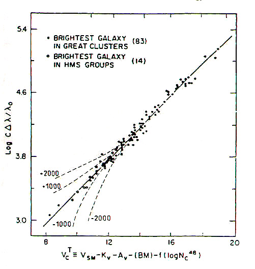
(0) Early canonical redshifts in the Hubble distance-redshift relationship:
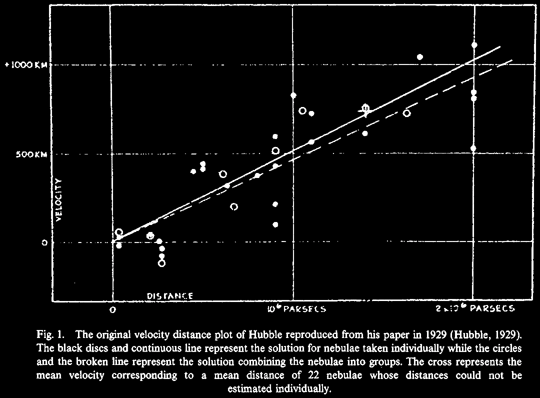
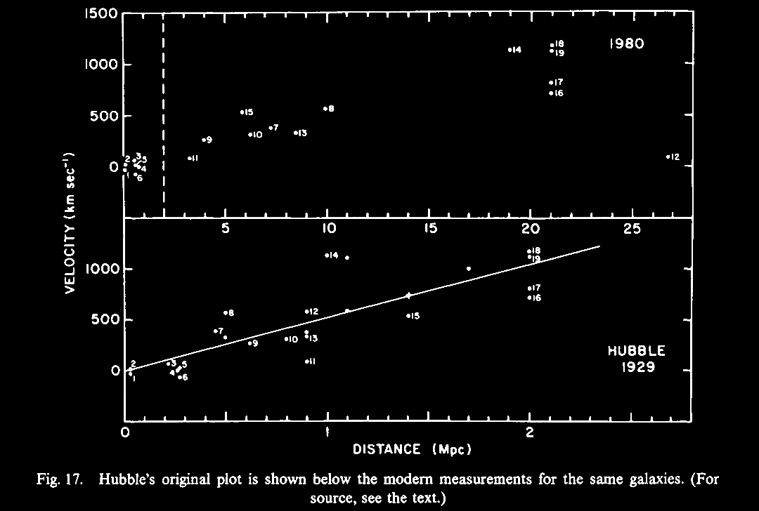
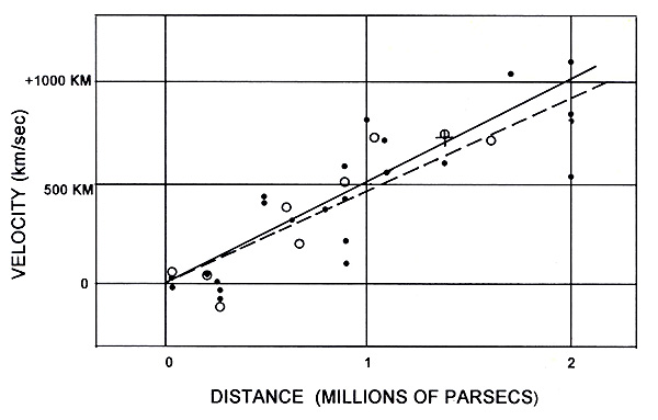 Hubble relation (Hubble, 1929; from Hoyle et al. 2000). |
|
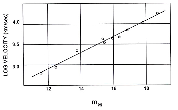 Log velocity plotted against photographic
magnitude (mpg) indicative of the
Hubble relation (Hubble & Humason, 1931; plot
taken from Tolman, 1934; from Hoyle et al.
2000).
Log velocity plotted against photographic
magnitude (mpg) indicative of the
Hubble relation (Hubble & Humason, 1931; plot
taken from Tolman, 1934; from Hoyle et al.
2000). 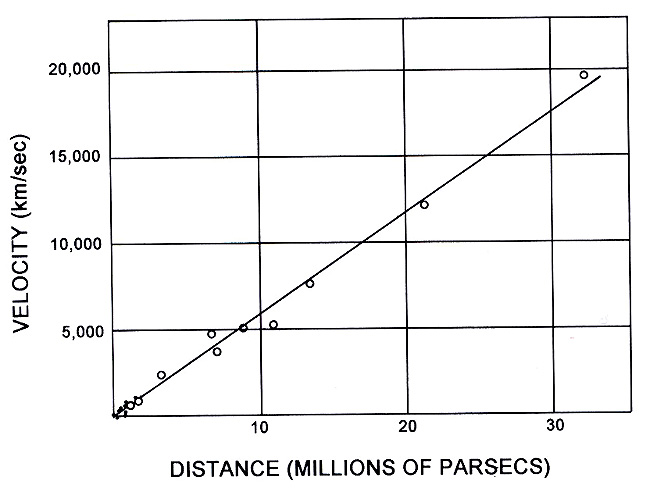
Hubble relation (Tolman, 1934; from Hoyle et al. 2000).
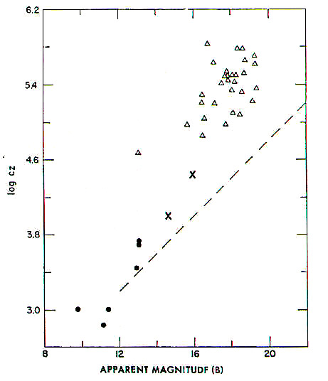
Some early (but not-understood) observations of this non-canonical or unexpected redshift scatter phenomena were compiled in the study of Lang et al. 1975 by plotting of galactic redshifts taken from the de Vaucouleurs, G. & de Vaucouleurs, A. 1964. Bright Galaxy Catalogue (Austin, TX: University of Texas Press; and since updated to a 3rd edition, 1994: https://heasarc.gsfc.nasa.gov/W3Browse/all/rc3.html). Among the 'bright' galaxies since the early 1960s there emerged a scatter of even the standard 'bright galaxies' in the de Vaucouleurs Catalogue.
Galaxy Radial Velocity (z in km s–1) versus
Apparent Magnitude (m). The data for this plot is taken
from Lang et al. (1975), from the 'Reference Catalogue
of Bright Galaxies' (de Vaucouleurs et al. 1964).
There is a high resolution PostScript version of this plot,
and the specific plot was created with Cat's eye (http://tarantella.gsfc.nasa.gov/viewer/example/catseye_intro.html).
In standard,
canonical, HBBC-compliant terms the scatter of redshifts was
interpreted as the peculiar velocities of the galaxies in a
cluster superimposed on the Hubble relation. However, that
effect is expected to dampen out and vanish with distance in
a standard interpretation. It does not.
Compiled by Allan Sandage, Palomar Observatories: Dashed lines
are supposed to represent the effect of peculiar velocities of
1000 - 2000 km/s (cited in Arp, 1998).
Compiled by Halton Arp (1968, cited in 1998), Max Planck
Institute: Solid circles = nearby Seyfert galaxies (gen.
spiral with very bright, rapidly varying nuclei); 'x's =
compact Seyfert-like galaxies; open triangles = QSOs; dashed
line represents predicted Hubble relation.
Redshift (v0) versus distance (Mpc): Ascending
Hubble relation according to Arp (1998).
By the early 2000s, the results were showing a scatter where the Cepheid distance ladder calculations showed galaxies nearer than indicated by their redshift (z) values. What was the meaning of these excess redshift values?
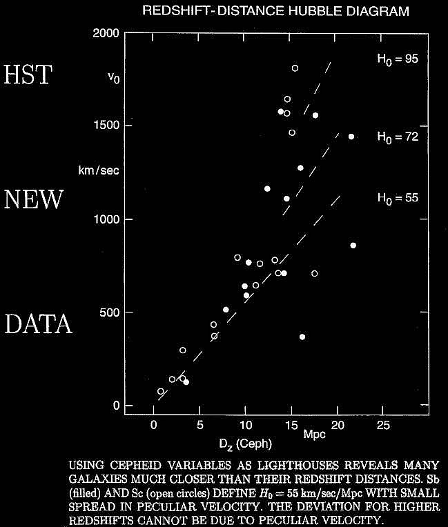
Based on data from the Hubble Space Telescope (www.haltonarp.org).
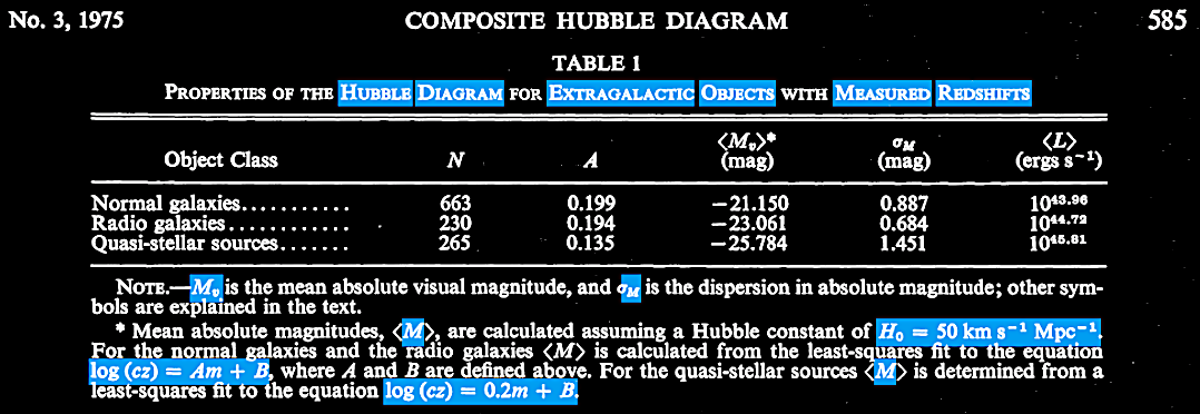
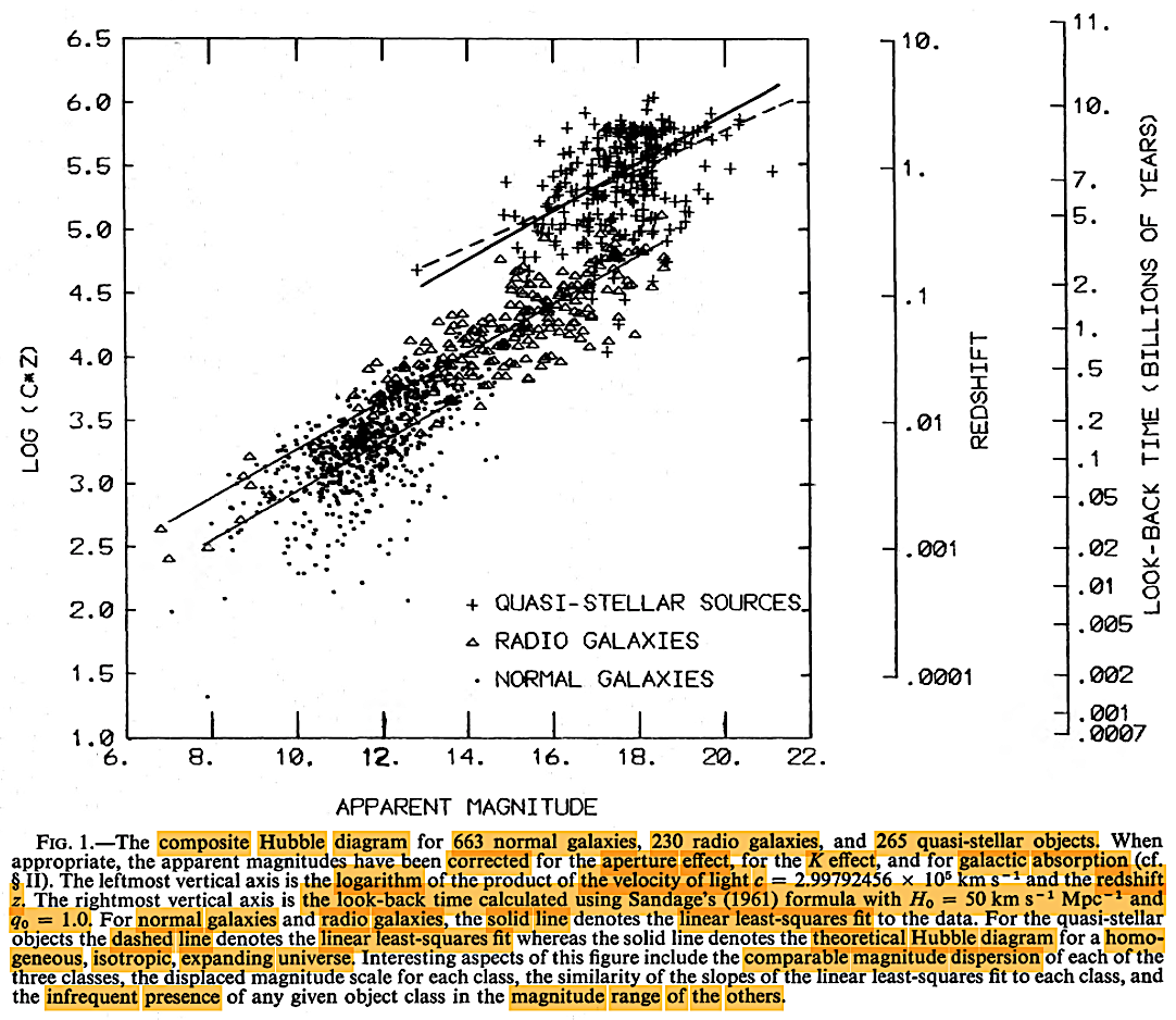
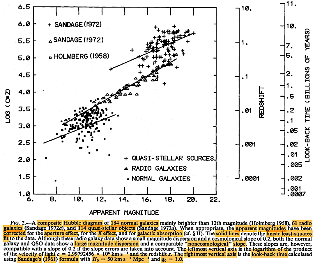
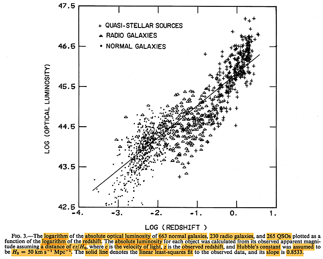
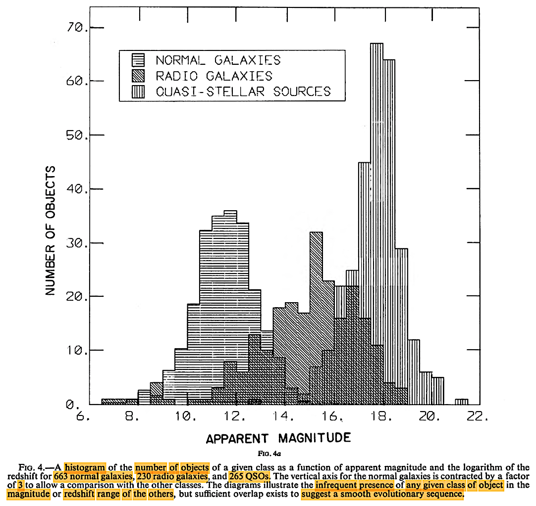
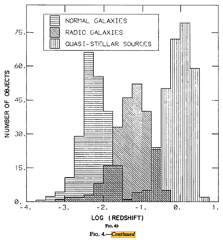
About a decade after the HBBC-CSSC controversy over QSOs, near the end of 1975, Lang, K. R. et al. published, The composite Hubble diagram. ApJ 202 (3), 583-590. https://articles.adsabs.harvard.edu/cgi-bin/nph-iarticle_query?1975ApJ...202..583, and sought to settle the issue in favor of evolutionary or HBB cosmologies by their analyses of the redshift situation among known QSOs as the situation stood nearly 10 years after the CSSC-HBBC-related arguments above. While they found showed an evolutionary sequence, it was not so much about the rival HBBC-CSSC models, but about the possible rival cosmogonies of galaxy evolution, as we shall see.
It is important to note that Lang et al. (1975) assumed the old Sandage and colleagues determined H0 = 50 km–1 Mpc–1 and a q0 = 1.0, when later H0 had jumped to nearly 70 km–1 Mpc–1 or higher (given the 'Hubble tension') and by 1998, the q0 parameter had switched sign to q0 = ~ –1, as discussed in chapter III and above, regarding the so-called 'accelerating Universe' or 'dark energy' discoveries.
 |
 |
 |
 |
Lang et al. (1975).
Lang et al. (1975) had indeed found an evolutionary sequence, but with the actual distances of the quasars not yet well-established, it was illusory as support for the HBBC, and as mentioned, it actually suggested something quite revolutionary as far as galactic cosmogony and evolution is concerned.
We turn to summaries of these emerging data showing a QSO scatter of redshifts.
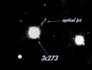
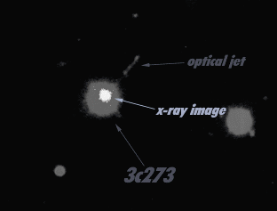
(http://chandra.harvard.edu/xray_sources/3c273/xray_opt.html).
Scatters in
redshifts appear not only in linear size vs luminosity but
also in redshift vs spectral index (Condon, 1991).
Linear
Size versus Luminosity 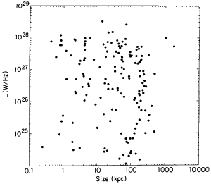 For 1.4 Ghz radio sources brighter that 2 jansky, the distribution of linear size versus luminosity is a scatter diagram (Condon, 1991). |
Redshift
versus Spectral Index 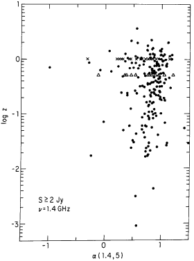 The distribution of redshift versus spectral index at 1.4 GHz is also a scatter diagram (Condon, 1991). |
Greer (in a
1999 presentation at a science & religion conference in
Gallup, NM) presented these quasar (QSO) redshift scatters
in redshift (raw z as well as log z) vs
apparent magnitude (m) data from Hewett, P. C.,
Foltz, C. B., & Chaffee, F. H. 1995. The large bright
quasar survey [LBQS]. 6: Quasar catalogue and survey
parameters. AJ 109 (4), 1498. https://articles.adsabs.harvard.edu/full/1995AJ....109.1498H;
LBQS home: https://heasarc.gsfc.nasa.gov/W3Browse/all/lbqs.html).
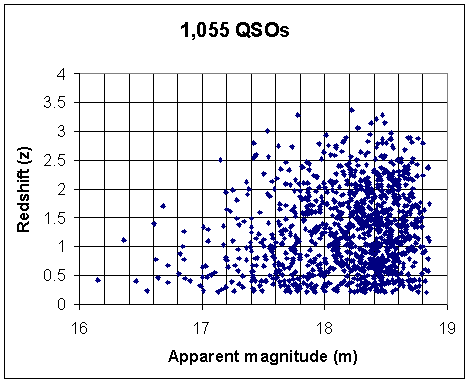 Compiled & graphed by L. Greer (1999) from the LBQS data (Hewett et al. 1995). |
|
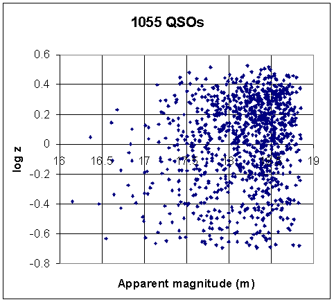
Excess QSO redshifts beyond
the Hubble relation for large galaxies (Joseph, 2010b).
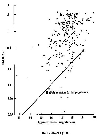
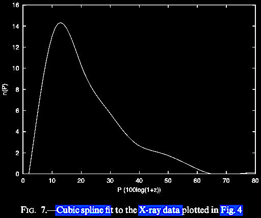
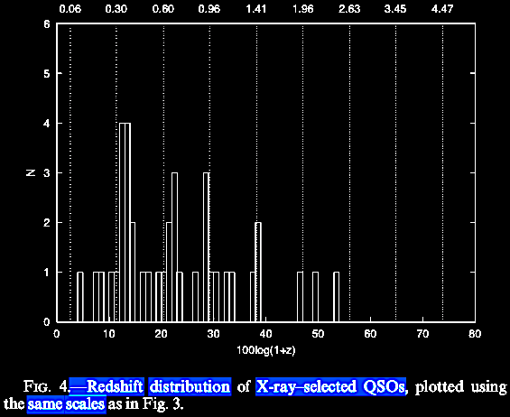
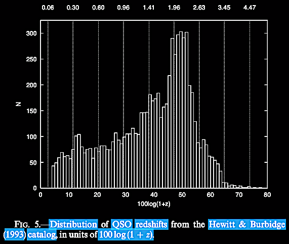
With a much larger data set Hoyle, Burbidge, & Narlikar (2000) in their volume presenting the QSSC the following year, quasars were shown to have a scatter instead of a good correlation with the Hubble distance relation:
The empirical relation: m = 5 log (z) + H0 (km s–1 Mpc–1)|
|
 Angular locations of the then-known 7315 QSOs projected on Milky Way Galactic coordinates (Hewitt & Burbidge, 1993; cit. in Hoyle et al. 2000). |

Further studies
confirmed an intrinsic excess of redshifts in certain AGNs,
such as QSOs and even radio galaxies. In pursuit of insights
from the Ambartsumian-Vorontsov-Vel'yaminov-Arp (AVVA)
cosmogony of ejection of higher redshift compact galactic
objects from lower redshift AGNs (see chapter IX),
Bell, M. B. 2007. Further evidence that the redshifts of AGN
galaxies may contain intrinsic components. arXiv release (v1
12 Apr 2007; v2 21 Aug 2007): https://arxiv.org/abs/0704.1631.
ApJ 667 (2), L129. https://doi.org/10.1086/522337,
referring to the DIR (declining intrinsic redshifts)
post-ejection evolving with increasing luminosity. According
to the DIR deductions from the Ambartsumian-Vorontsov-Vel'yaminov-Arp (AVVA)
cosmogony young AGNs or QSOs evolve into BL Lac objects,
Seyfert galaxies, and in the penultimate stage into radio
galaxies before losing the rest of their intrinsic redshift
and becoming quiescent mature galaxies. Because of low
redshift galaxies and high redshift compact sources, we can
now infer that the evolutionary pattern Lang et al.
espied in 1974 does not show the evolutionary BB cosmology,
but the stages of the Ambartsumian-Vorontsov-Vel'yaminov-Arp
(AVVA) cosmogony of galaxies (see chapter
IX), and a brief introduction below.
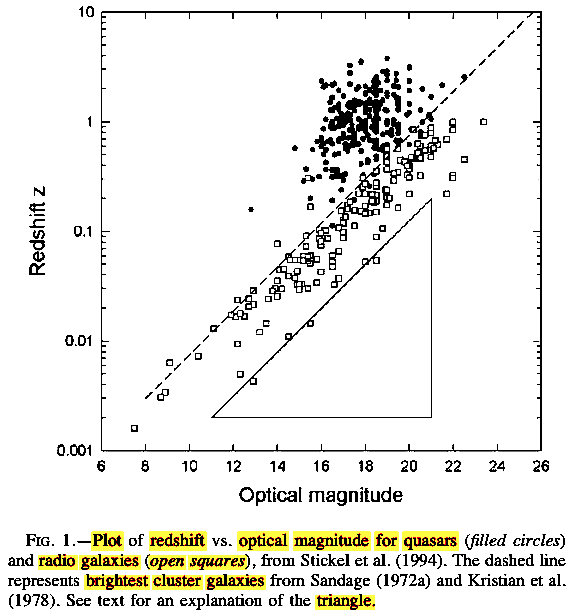 The triangle at the
lower right pf Figure 1 represents where the QSOs
would be if the intrinsic component were absent.
|
 |
The intrinsic
redshifts of AGNs suggest that we should expect increased
departures from the ordinary H0 redshift
relation perhaps with the degree of the energetic activity of
AGNs.
Although the QSOs and
other types of AGNs attracted more attention, some little
noticed papers showed evidence for intrinsic (non-canonical)
redshifts in regular spiral galaxies: Russell, D. G. arXiv: v1
19 Aug 2004; v2 26 Sep 2004: https://arxiv.org/abs/astro-ph/0408348); 2005. Evidence for intrinsic
redshifts in normal spiral galaxies. Astrophys Space Sci
298, 577. https://doi.org/10.1007/s10509-005-2317-x.
Russell summarized data showing that even ordinary spiral
galaxies have some excess redshift component, above the Hubble
constant redshift-distance relation expectations. In his 2004
arXiv manuscript, Russell had diagrams to show this, including
some intrinsic additional redshift seemingly dependent in part
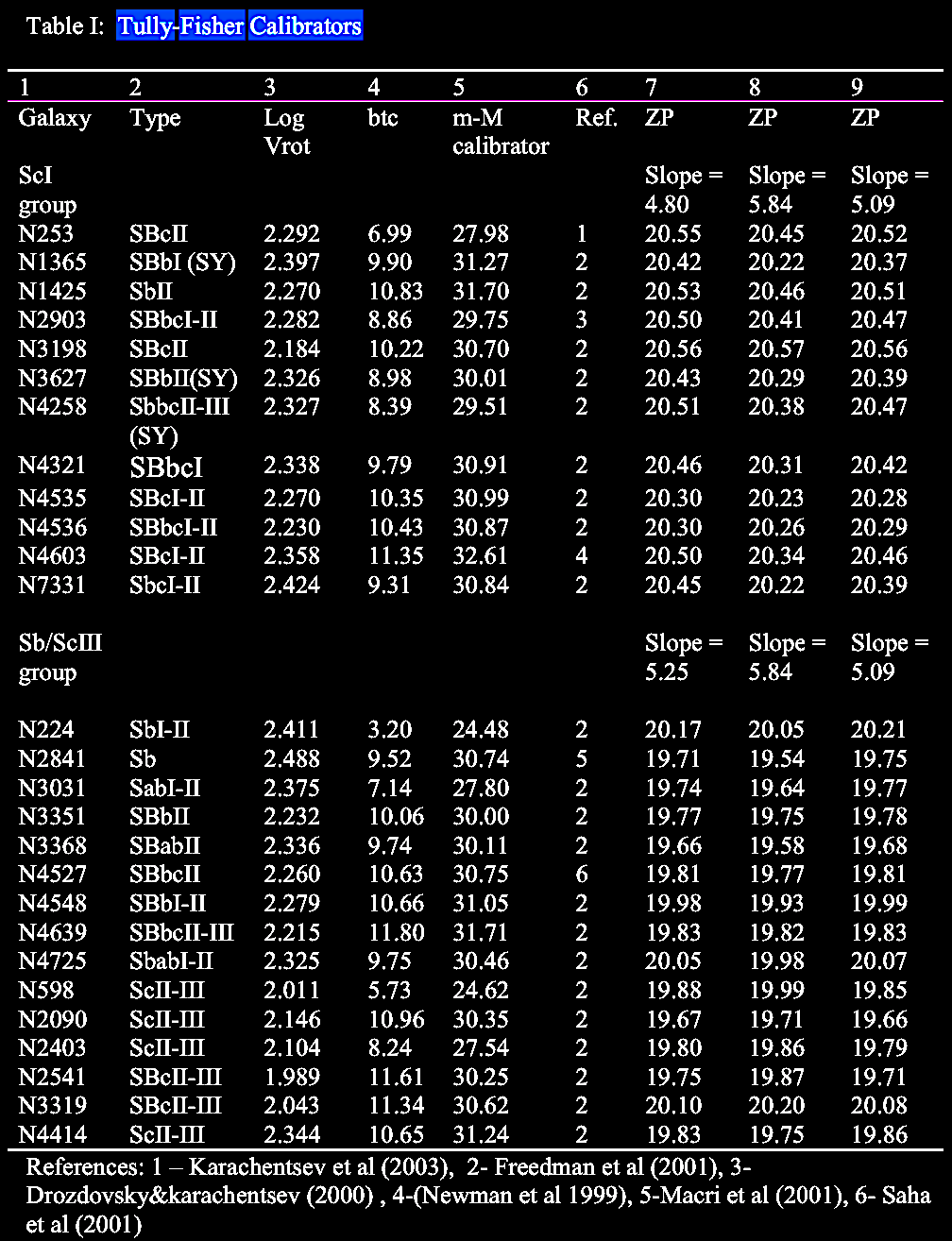
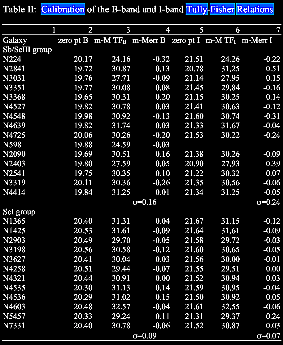
on morphology, calibrated by the commonly-used Tully-Fisher
relation (link)
between mass / intrinsic luminosity (of spiral galaxies) vs.
asymptotic rotation velocity (expressed as emission line
width).
 |
 |
 |
 |
 |
 |
 |
 |
 |
 |
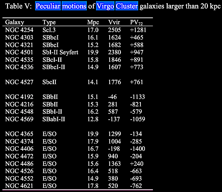 |
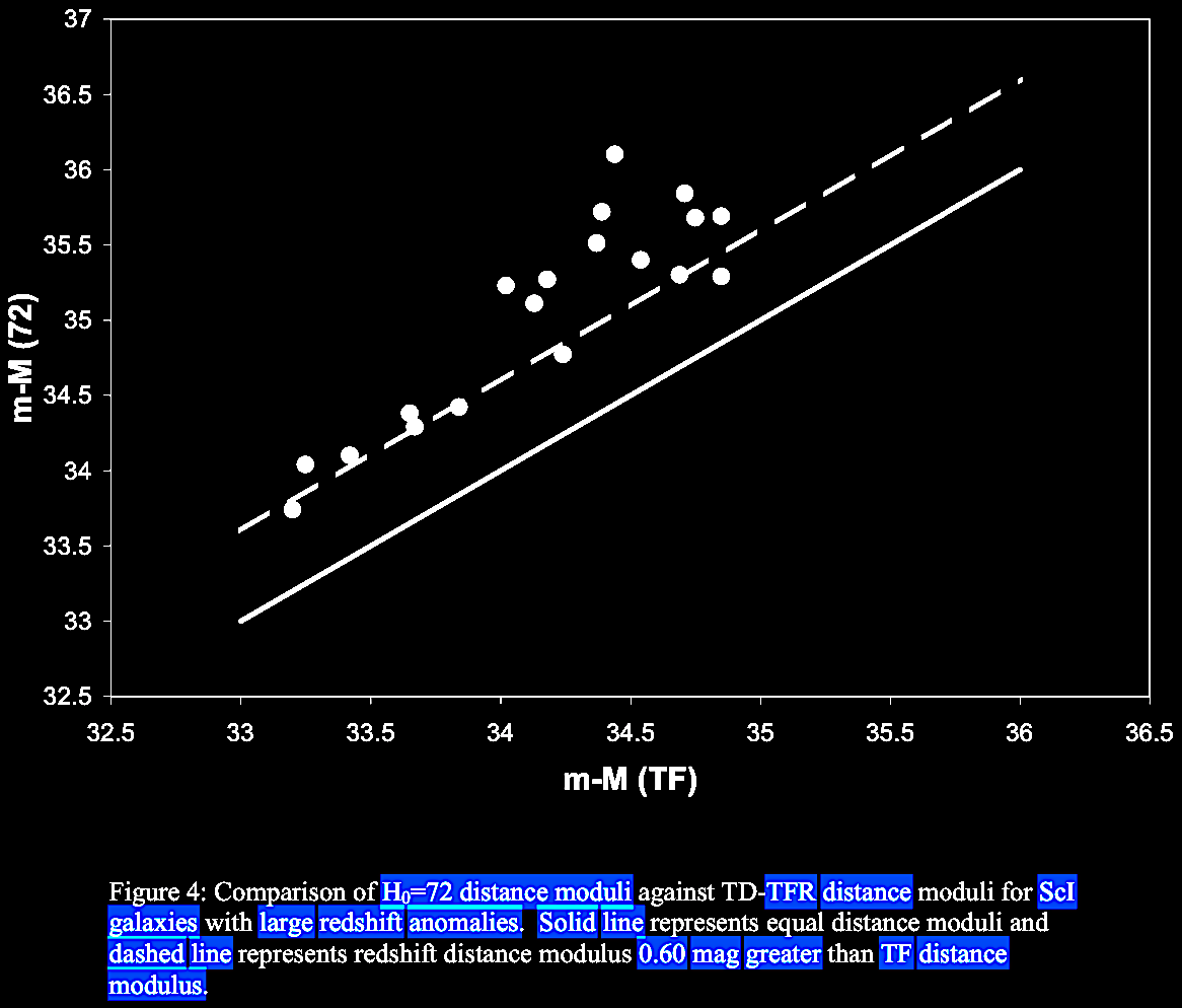
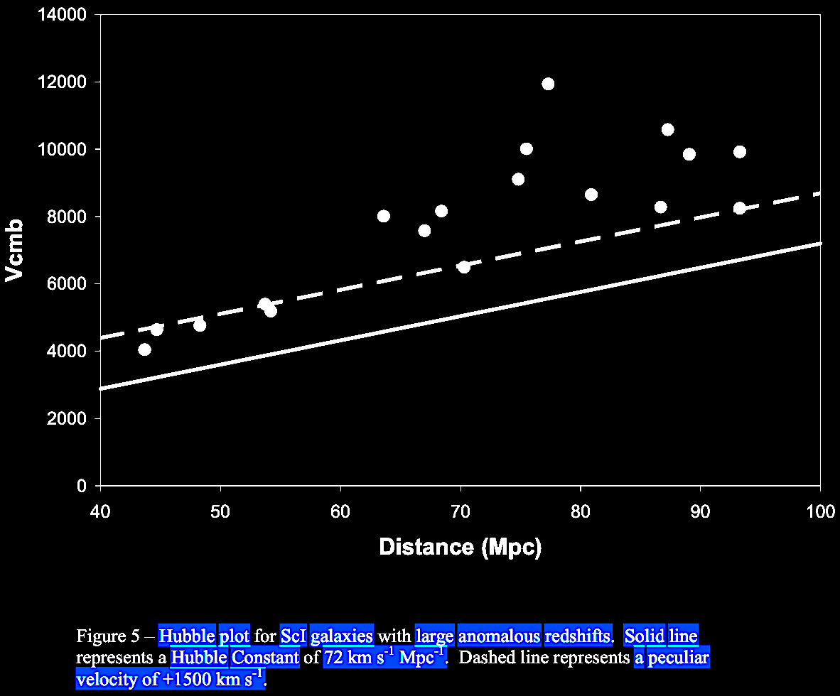
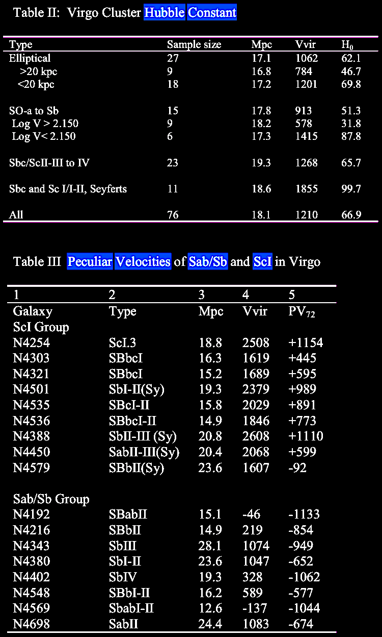
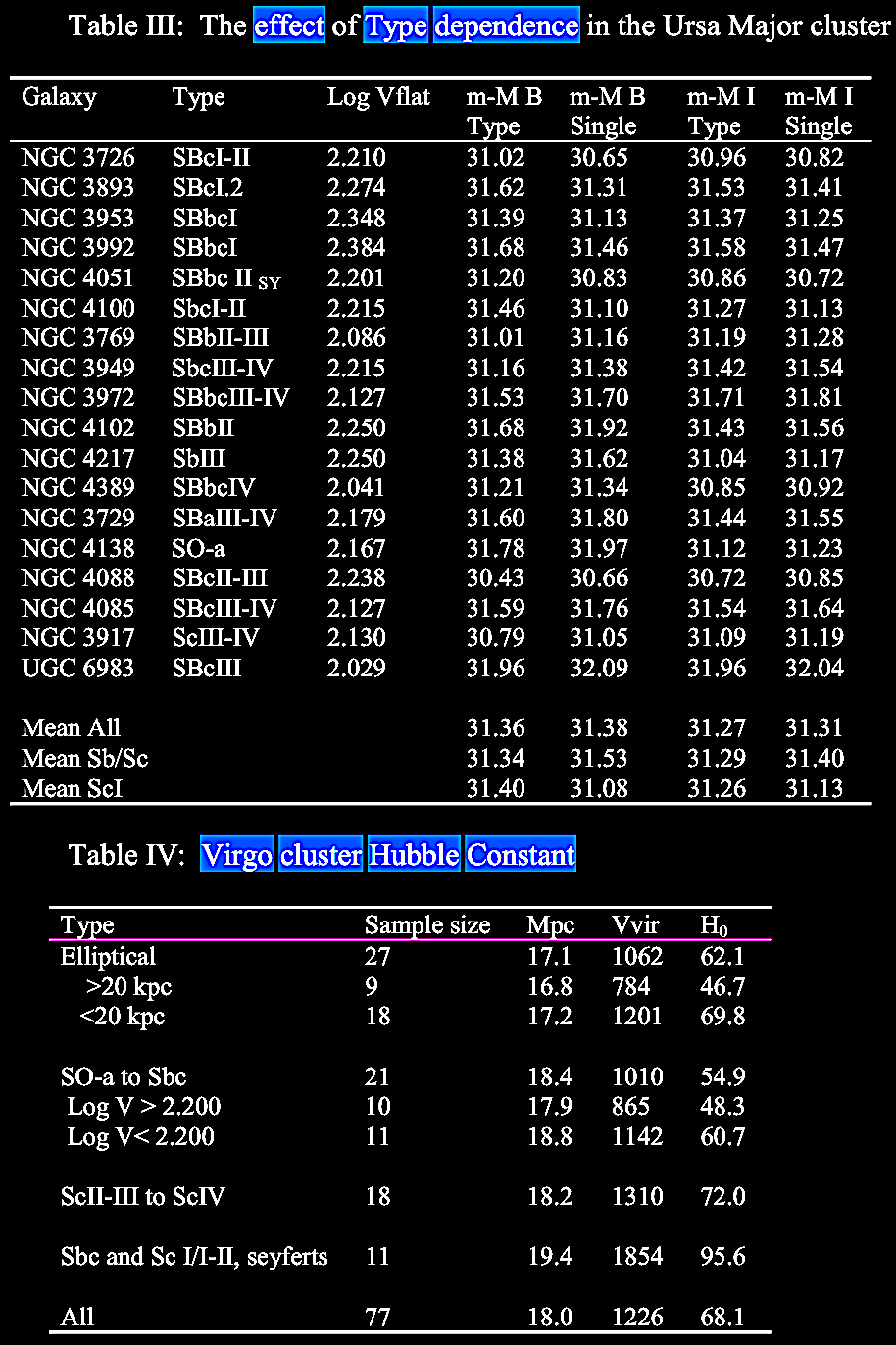
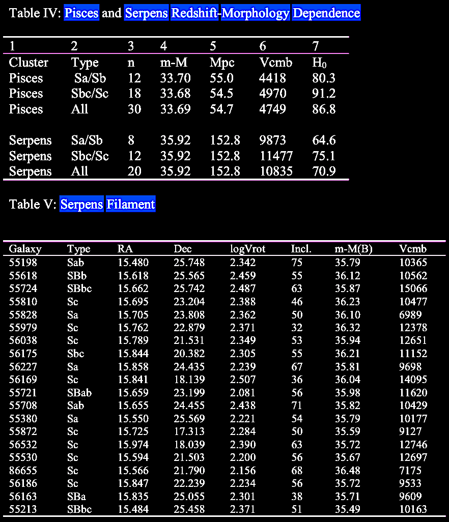
In Table
VI in the next two cells below, the barred spiral ScI
data are of especial interest since they include the
largest cohort of the barred spiral galaxies in the
study. |
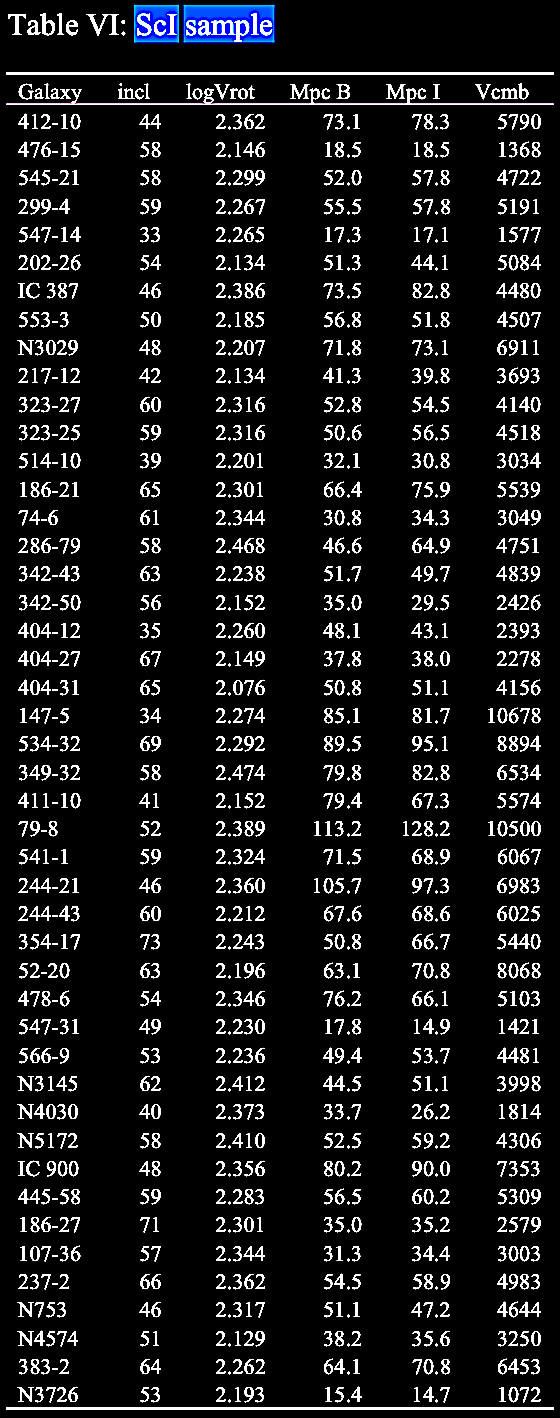 |
Table VI:
ScI sample (cont.).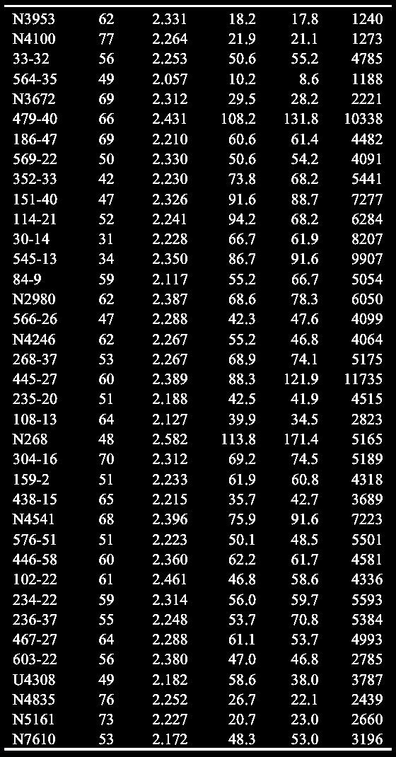 |
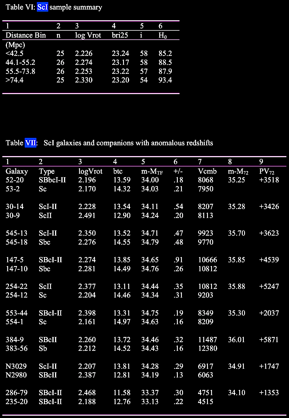 |
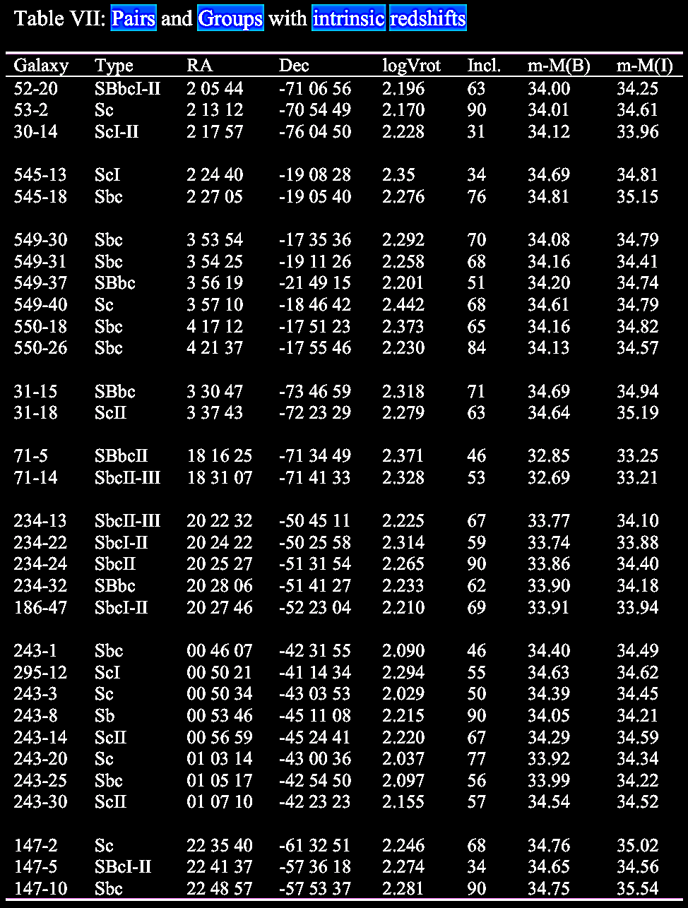 |
 Table VIII. Excess redshifts of small groups (cont.).  Excess or intrinsic redshifts associated with small groups of galaxies. |
 |
 |
 |
Next, we turn to
divergent redshift associations and the early hypothesis of
galactic ejection phenomena, which will be discussed in depth
in later chapters.
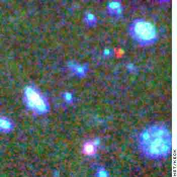
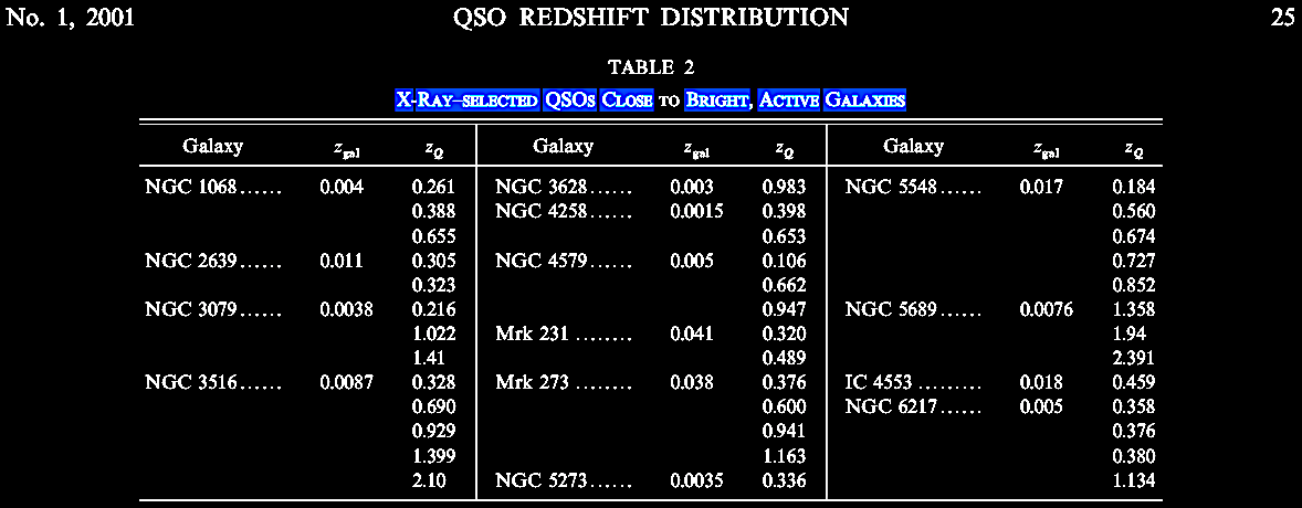
Furthermore, quasars began to be found in close apparent connection with nearby, lower redshift galaxies. Low redshift, barred spiral galaxy NGC 1073 with three putatively associated, high redshift QSOs (discovered by H. Arp; cited in Burbidge et al. 1999). Note the alignment of the quasars with the spiral arms. We will return to this and similar associations. These ejection phenomena data will be explored further in Chapters IX (Vast jets and galactic ejection phenomena: Mass origin-ejection?) and X (Multiple galactic alignments: Ejections and galaxy clusters?).
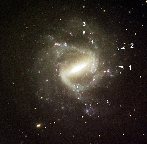
(Arrows added to image from http://www.astronomy.com/asy/default.aspx?c=a&id=3430).
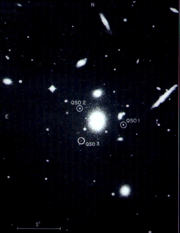
Another local, low redshift galaxy, NGC 3842, with three putatively-associated, more high redshift QSOs in juxtaposition (discovered by H. Arp; cited in Burbidge et al. 1999).
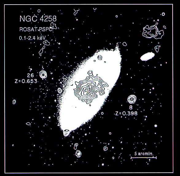
Higher redshift with nearly identical z-values, blue stellar objects in paired-alignment across the minor axis of the Seyfert galaxy NGC 4258 (cited by Arp, 1998 and Burbidge et al. 1999).
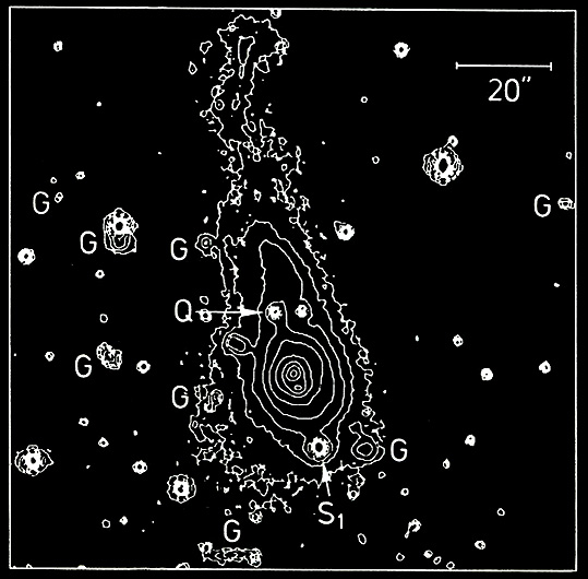
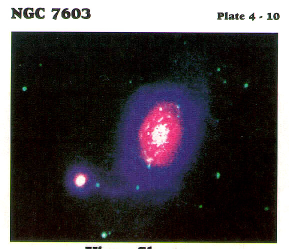
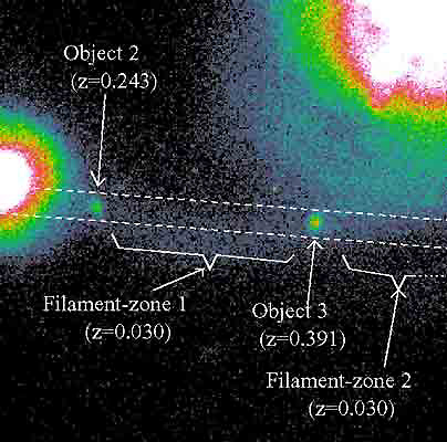
In 2002, two more high z objects were discovered in the NGC 7603 system, apparently associated with the same seeming ejection filament (Lopez-Corredoira & Gutierrez, 2002; https://doi.org/10.1051/0004-6361:20020476) indicating a decrease in z with distance from 'parent' galaxy (z = 0.391, 0.243, 0.057).
NGC 7603 & companions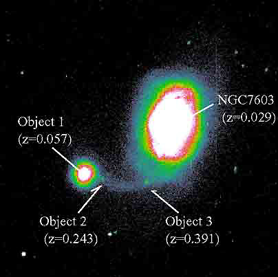 |
 |
There is an observed pattern as illustrated in the redshift vs. angular separation for 392 galaxy-QSO pairs plotted on a logarithmic scale (Left figure in the following table), indicating an inverse relation between (ascending) angular measure and (descending) redshift, strongly indicative of ejection and at least some connection between higher z values and proximity to putative ejections / angular distance 'associations.'
Hatched
regions indicate areas excluded by selection effect,
i.e., determining whether a galaxy-QSO 'pair' is
actually observed.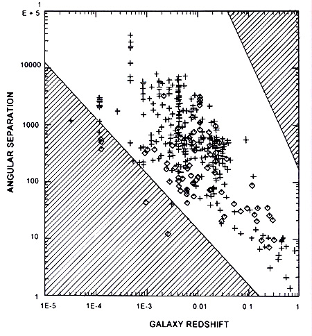 |
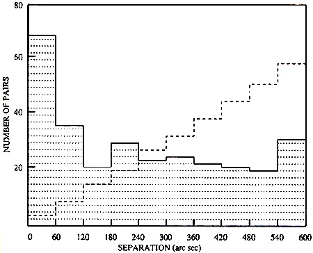
In another study, about
300 galaxy-QSO pairs were plotted by angular
separation (modified from Burbidge et al.
1990; Narlikar 1993). The dotted line indicates what
would be expected from a random background
distribution of QSOs without any pairing or galaxy-QSO
associations. |
In
yet another study, 197 galaxy-QSO pairs were plotted by
angular separation, and again, the non-random pattern of
association was assayed (Burbidge et al., 1990;
Hoyle et al. 2000).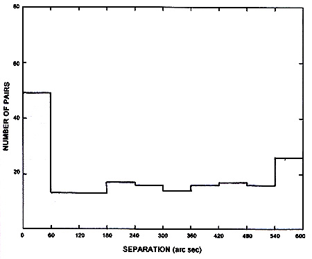 |
We will return to the recurring anomalous associations of low redshift galaxies, often with active galactic nuclei (AGNs), with higher redshift companion galaxies and galactic objects. These are often associated in ways which strongly suggest ejection and recurring ejection events. See Chapter IX. Vast jets and Galactic Ejection Phenomena: Mass origin-ejection?.
Another anomalous redshift phenomenon?
  A distant galaxy, STIS 123627, apparently had a changing redshift interpreted as 12.1 Gly distant down to a nearer 9 Gly (Joseph, 2010a). If this is real, it is again more evidence of a non-distance related z values. |
(iv) Unusual
redshift periodicities which won't go away.
[Image from Burbidge, G. 2003. NGC 6212, 3C 345, and other Quasi-stellar Objects associated with them.
ApJ 586, L119. https://iopscience.iop.org/article/10.1086/374793/fulltext/16874.text.html#crf14].
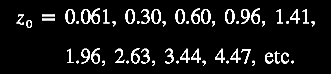
Brief Excursus on the Ambartsumian-Vorontsov-Vel'yaminov-Arp (AVVA) galactic ejection cosmogony hypothesis (for more, see forthcoming Chapter IX). Cf. Arp, 2003. Catalogue of Discordant Redshift Associations; pp. 13-16. The clustering of redshift quantities around certain "preferred values" was discovered by Burbidge & Burbidge (1967. Limits to the distance of the Quasi-Stellar Objects deduced from their absorption line spectra. ApJ 148, L107. https://www.adsabs.harvard.edu/full/1967ApJ). K. G. Karlsson (1971. Possible discretization of quasar redshifts. Astron. Astrophys. 13, 333. https://adsabs.harvard.edu/pdf/1971) showed that these discrete values follow an empirical relationship, (1 + z2) / (1 + z1) = 1.23, where z1 = the lower redshift and z2 = the next higher redshift up (Arp, 1998. Seeing Red: Redshifts, Cosmology, and Academic Science. Apeiron Press; p. 203) yielding preferred redshift peaks or periodicities in a geometric series or Karlsson series, where z1 = or corresponds to zi and z2 = or corresponds to zi + 1, with terms reordered thus:
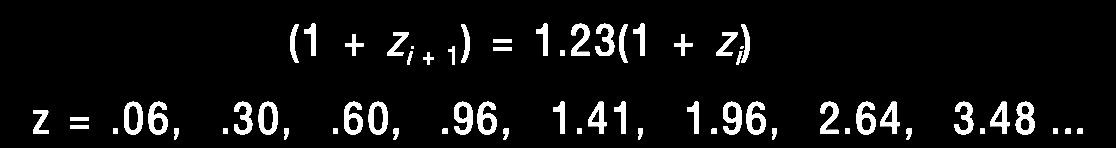
Karlsson showed that the first six elements of the series were observed in the available redshift data, and further he predicted the existence of the next higher peaks with values of z = 2.64 and 3.48. So, given that we repeatedly observe pairs of quasars or other higher redshift compact objects juxtaposed across the minor axis of lower redshift active galaxies as if ejected in pairs from the putative parent galaxy with its lower redshift (zG), suppose that we consider the putatively ejected pair of quasars with their measured redshifts (z1, z2) for example across NGC 4258 (in the figure above from Burbidge & Burbidge, 1997. Ejection of matter and energy from NGC 4258. ApJ 477, L13-L15. https://doi.org/10.1086/310517, which is discussed in greater detail in chapter V), we can relate them to the parent galaxy redshift (zG) by correcting their redshifts to be in the reference frame or rest frame of the active center of the parent galaxy (zG), i.e., zQ, related by (1 + zQ) = (1 + z1) / (1 + zG). The difference between zQ and the next Karlsson peak in the series is assumed to predict the actual velocity of ejection, vej in units of c, that is, (1 + vej) = (1 + zQ) / (1 + zp), where zp = the redshift of that nearest Karlsson periodicity peak. For more details see forthcoming Chapter IX.
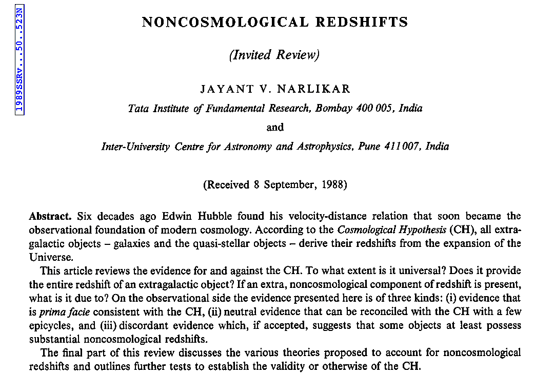
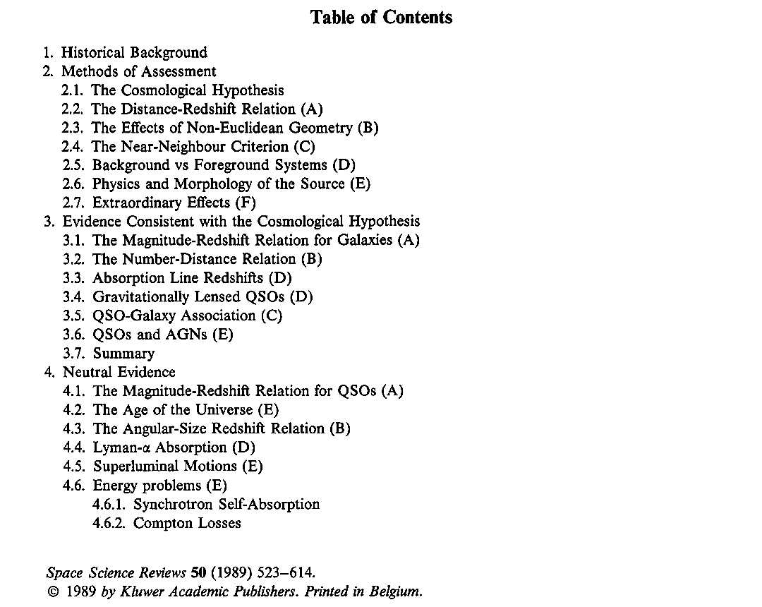
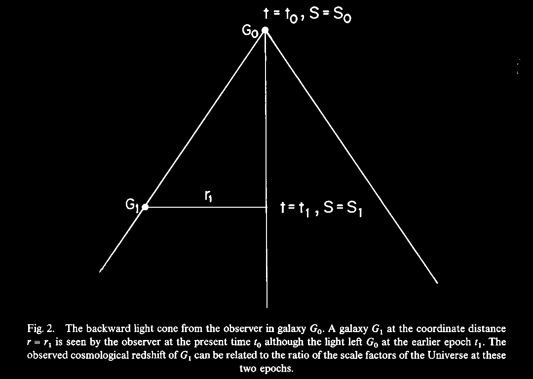
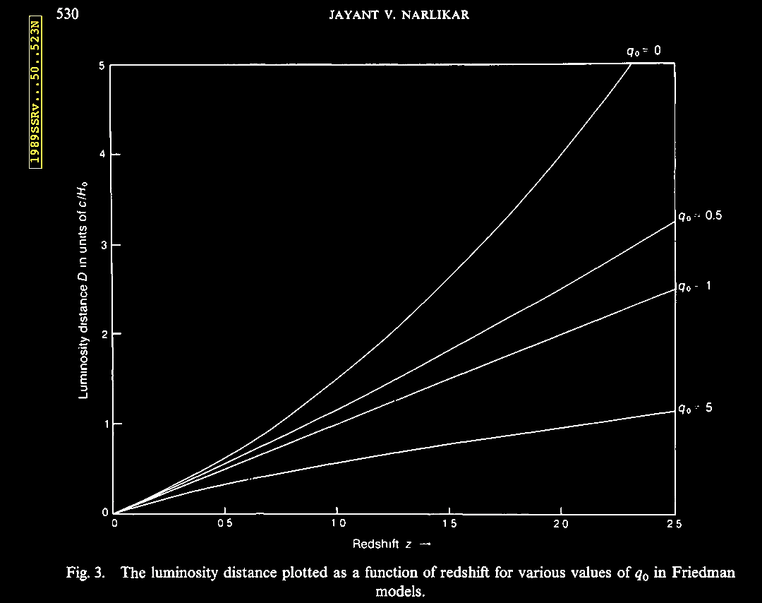
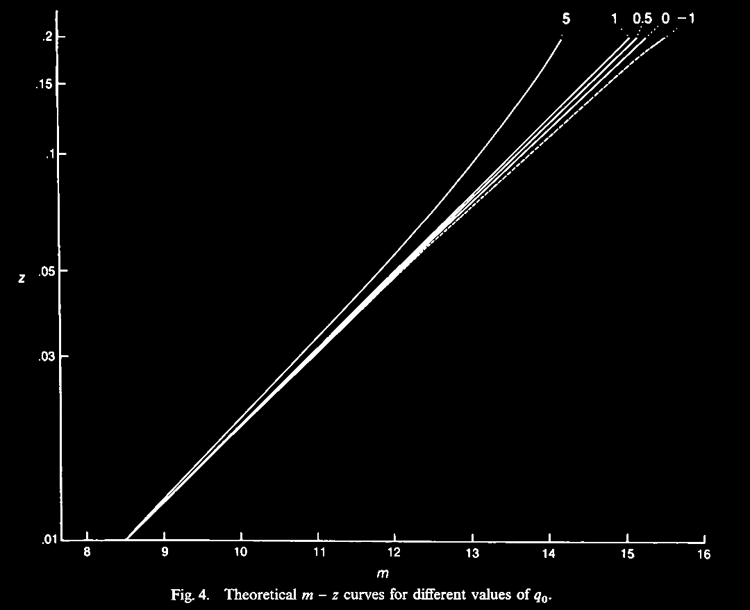
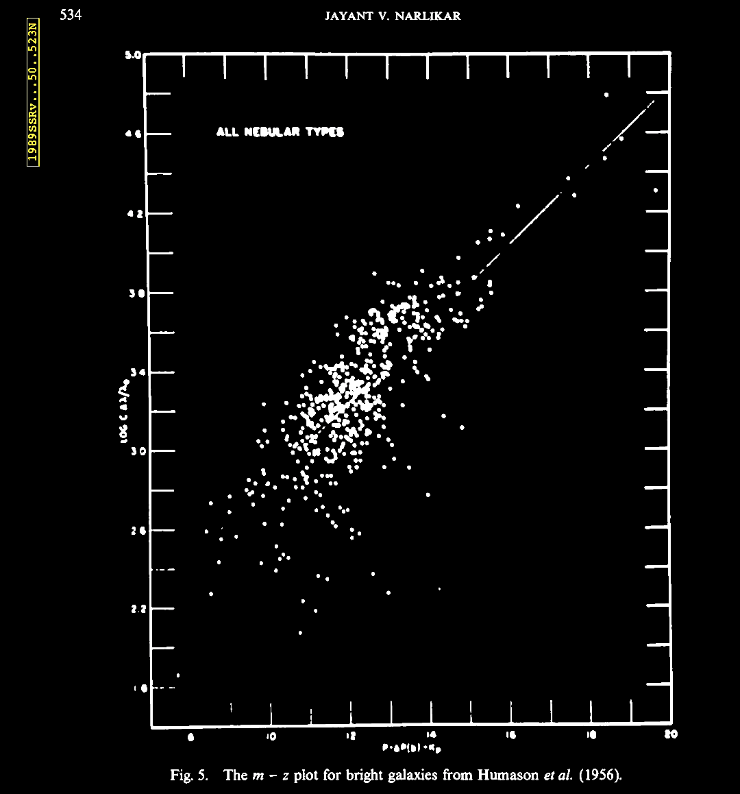
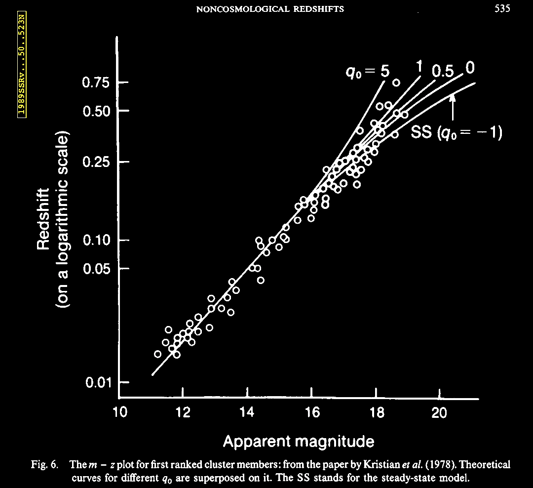
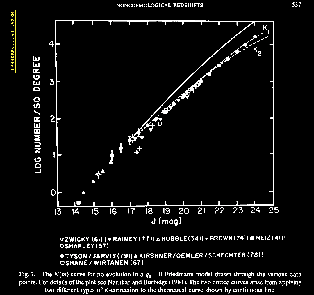
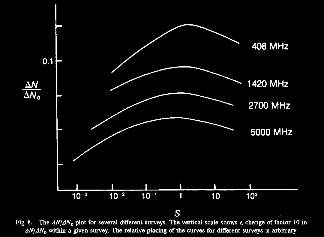
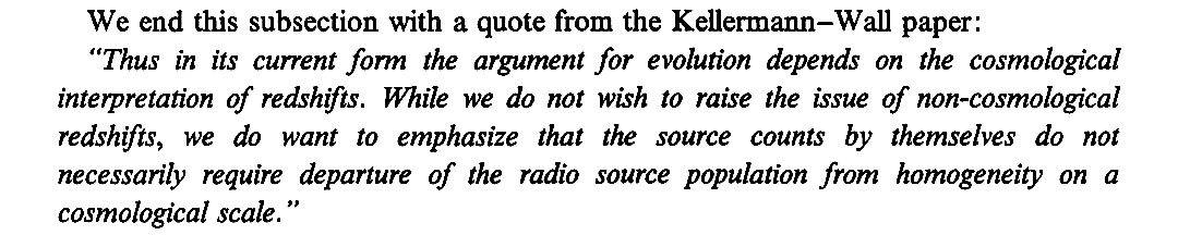
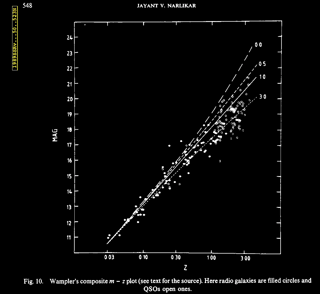
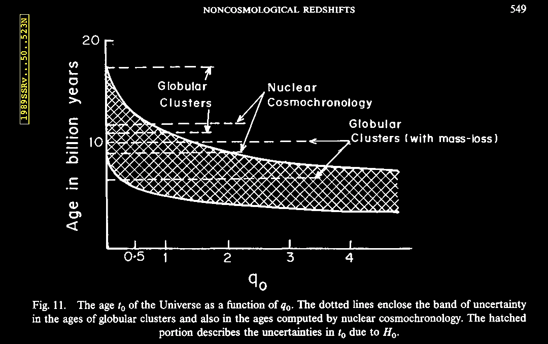
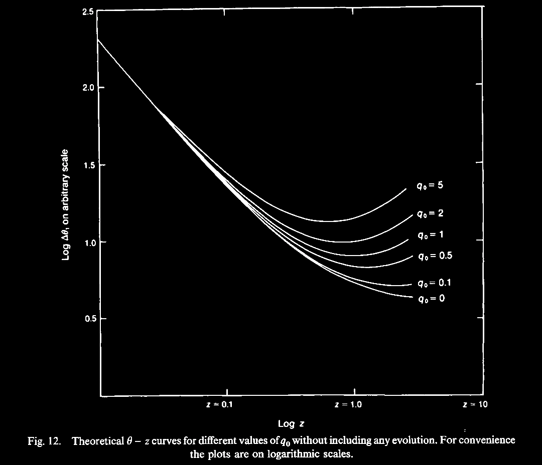
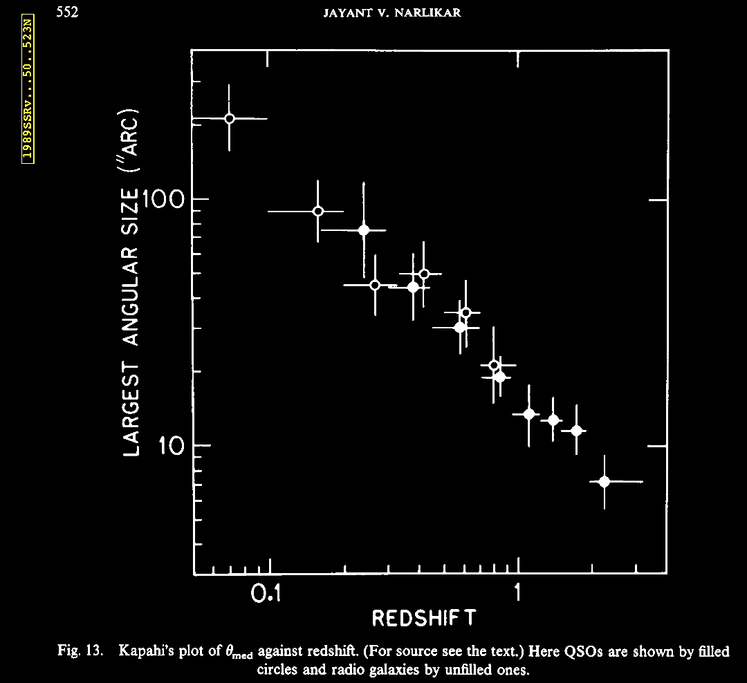
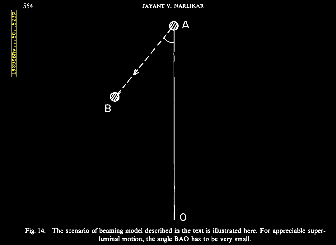
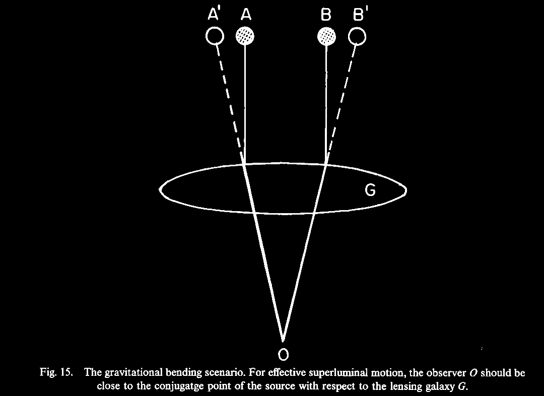
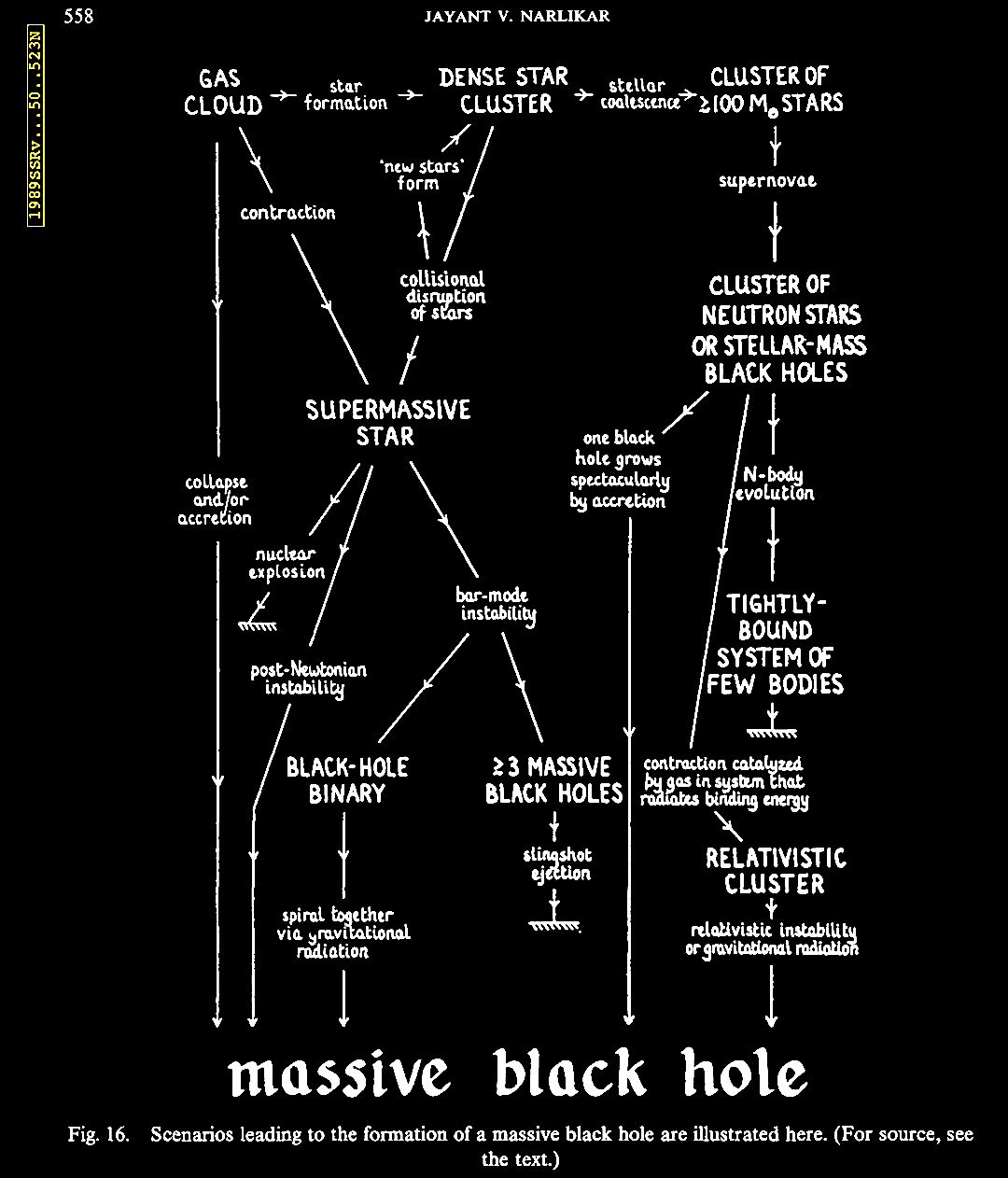
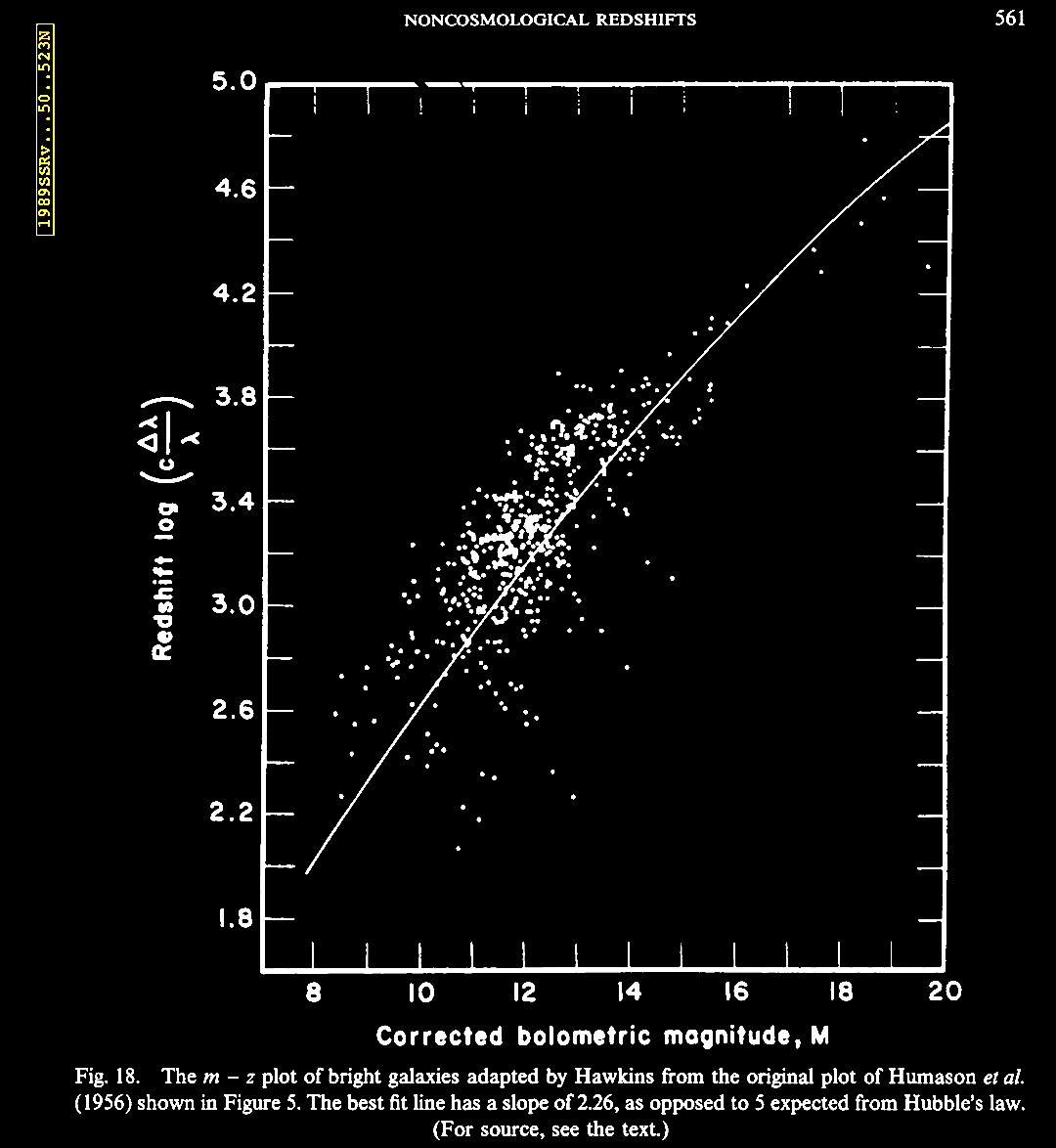
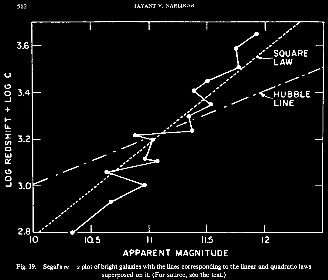
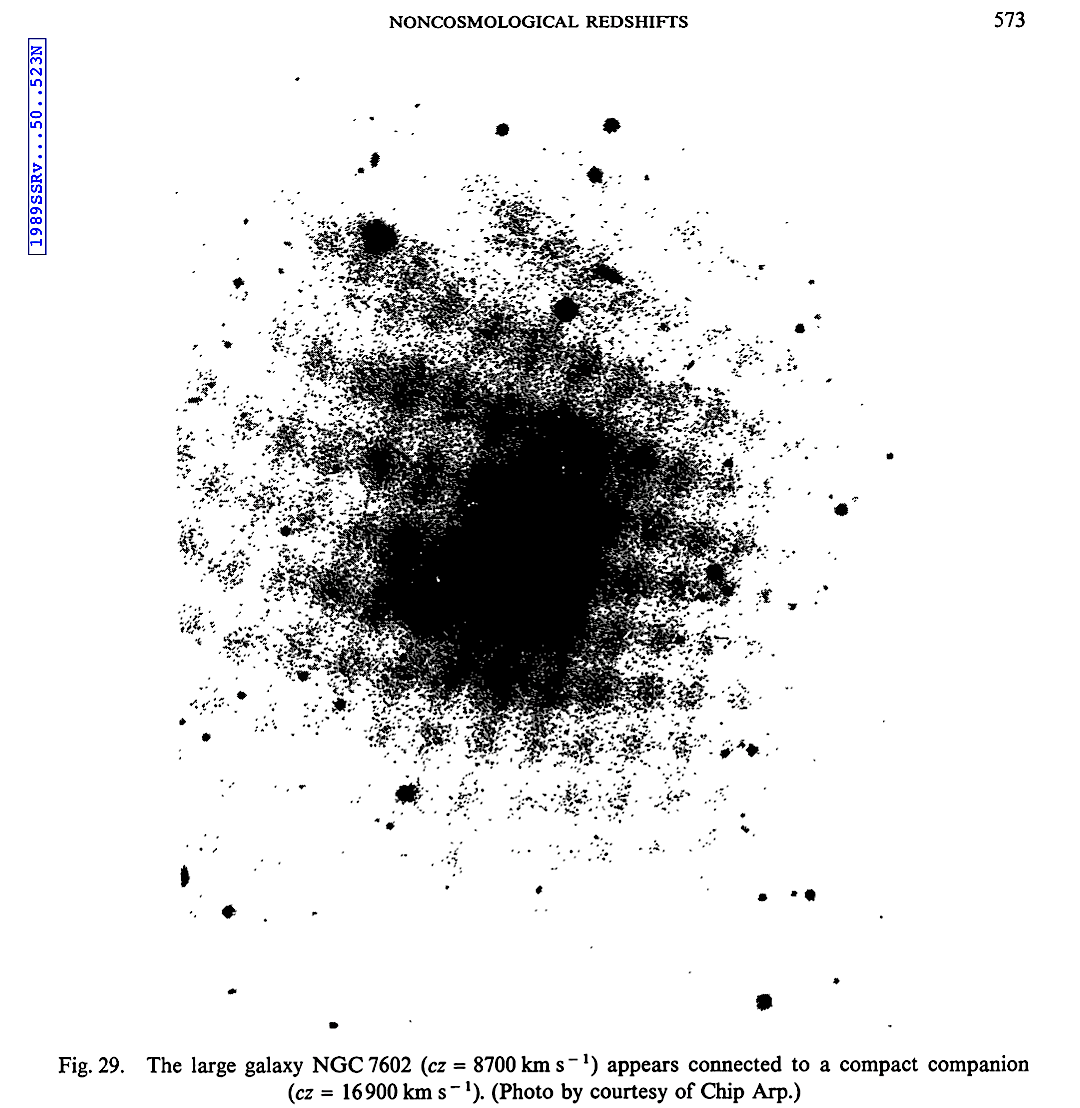
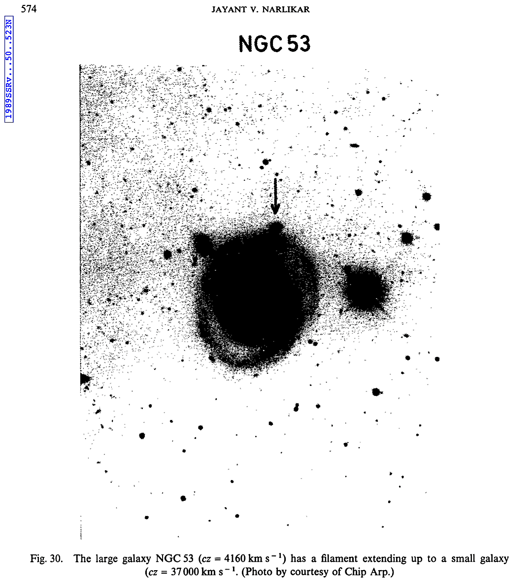
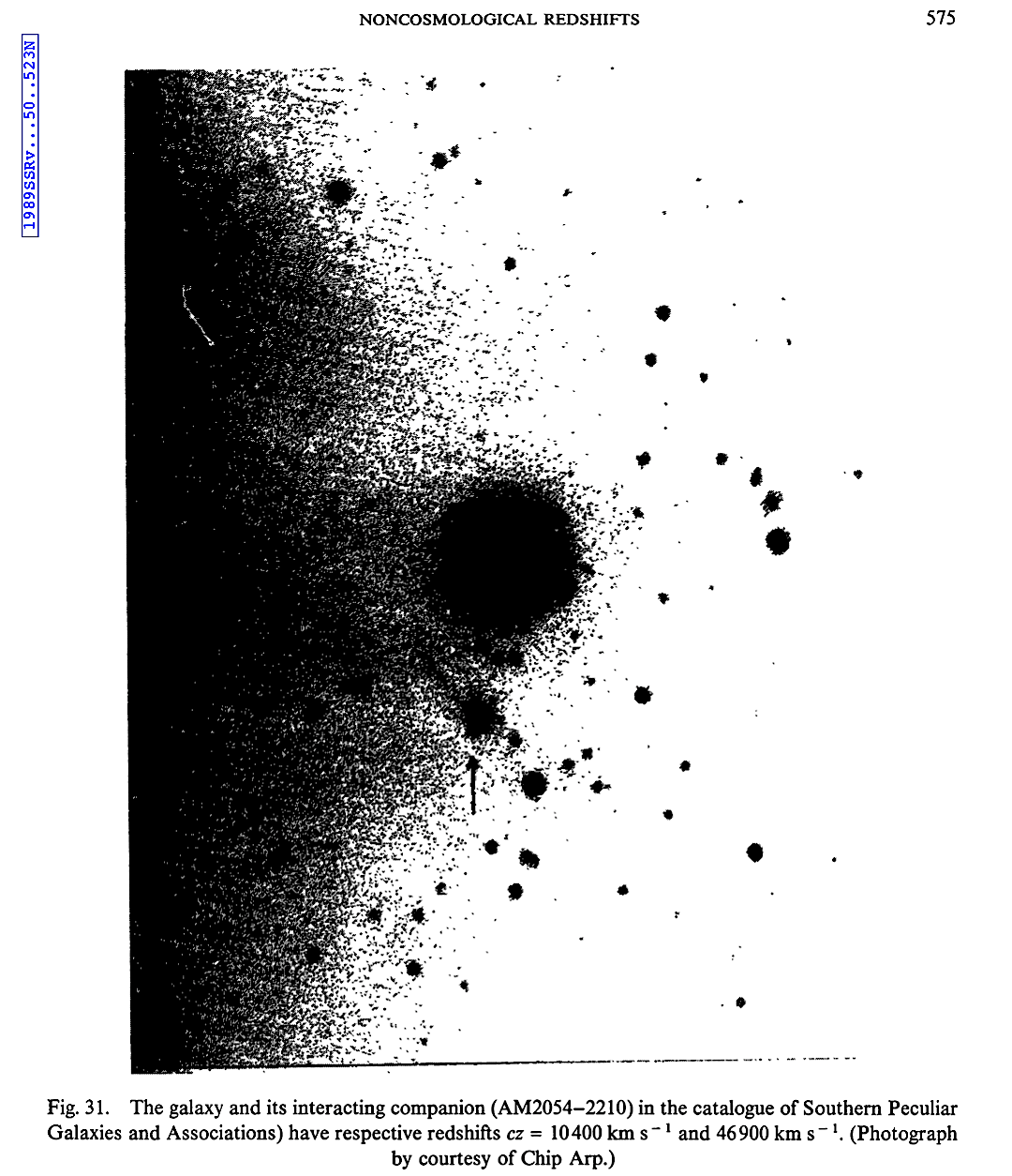
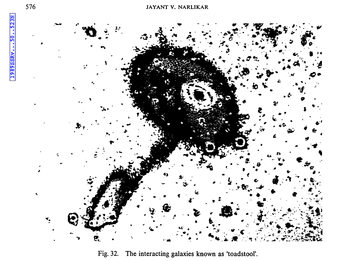
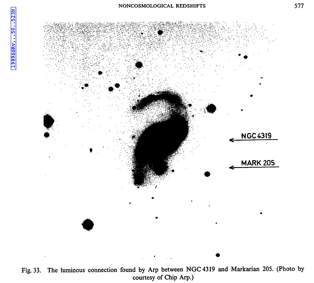
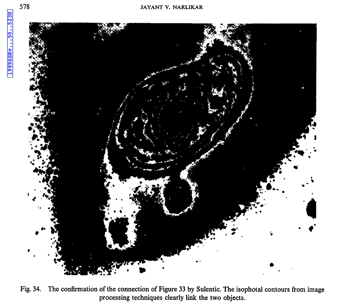
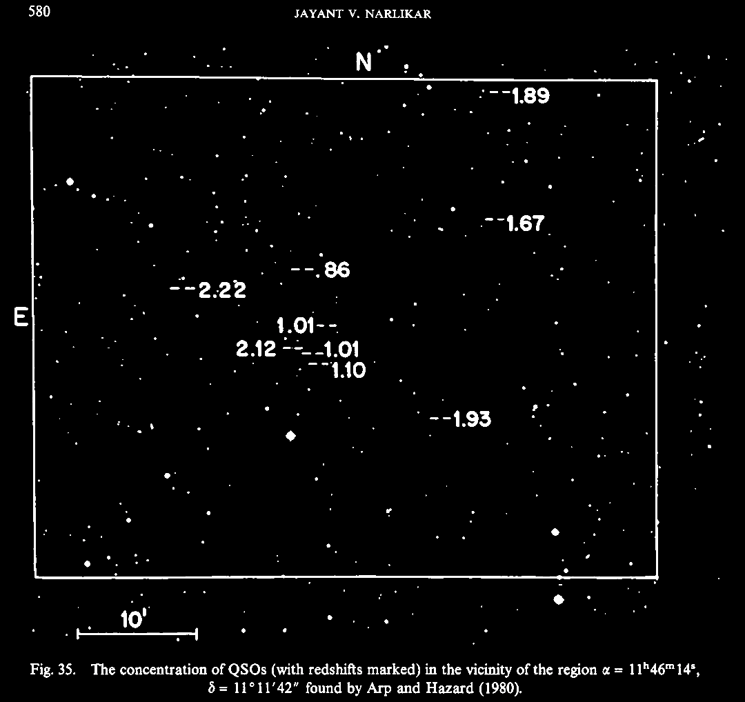
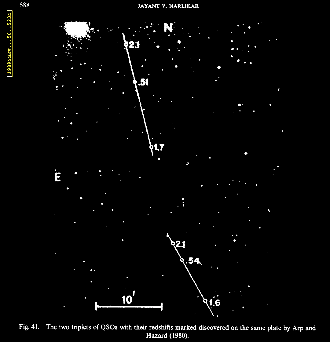
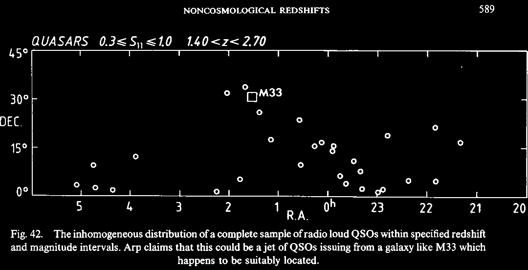
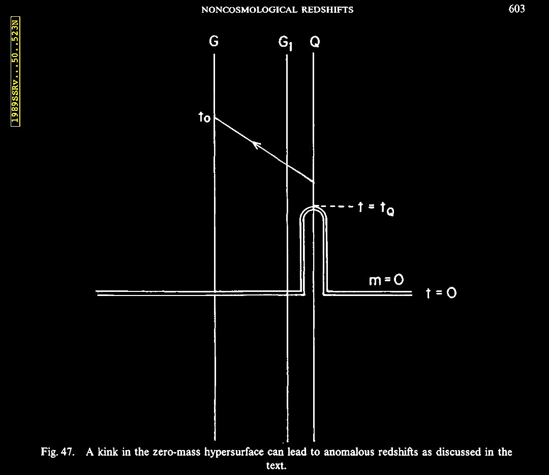
In 1989, Jayant Narlikar was invited to review the issue of 'noncosmological' or non-Hubble relation associated redshifts, and he also covered some of the hypotheses and a few theories put forward to explain these 'anomalous' data. Narlikar, J. V. 1989. Noncosmological redshifts (Invited Review). Sp. Sc. Rev. 50, 523. https://articles.adsabs.harvard.edu//full/1989SSRv...50..523N/0000538.000.html. Narlikar reviewed the history of the discovery of cosmological redshifts, which abide by the 'cosmological hypothesis' (CH) of an expanding Universe, as well as of the non-Hubble relation or 'anomalous' redshifts, and the attempts to interpret these data. Already multiple examples were known then (1989), and much more has been found since. We turn aside to consider this historic review from late in the 20th century. A forerunner of this review was a lecture given by Prof. Narlikar in 1986 at an IAU symposium, followed by a revealing discussion about how the subject was received at the meeting (Narlikar, J. V. 1986. Noncosmological Redshifts. Symposium - International Astronomical Union 119, 463-473; also In Swarup, G. & Kapahi, V. K. (eds.). Quasars, pp. 463-473. https://doi.org/10.1017/S0074180900153215).
 |
 |
 |
 |
 |
 |
 |
 |
 |
 |
 |
 |
 |
Then
about 2 decades, and now many decades, of data
collection show that QSOs do not have a linear
Hubble relation, but remain an anomalous scatter
diagram. 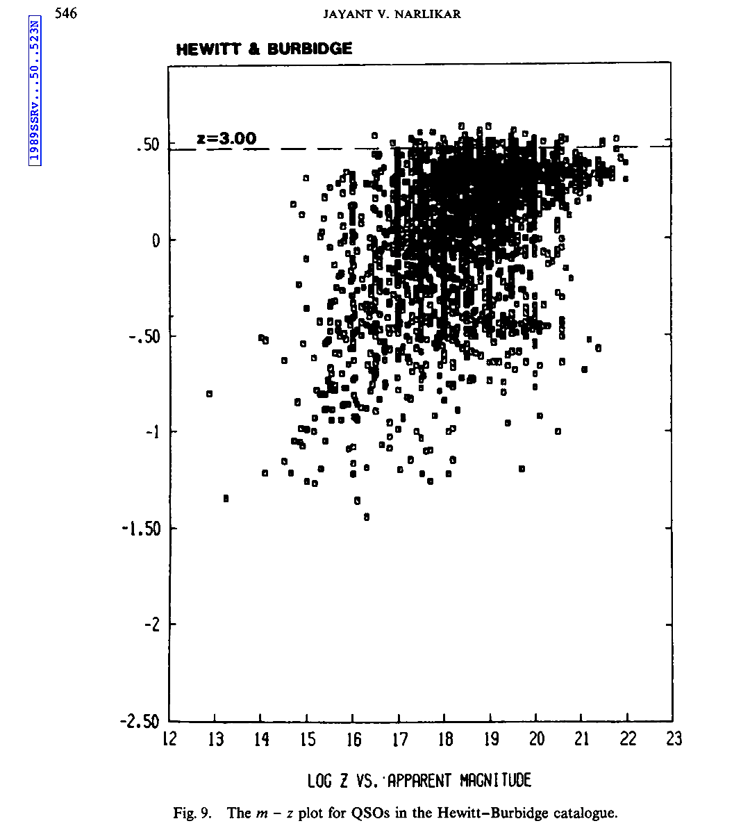 |
 |
 |
 |
 |
 |
 |
 |
 |
 |
 |
Now,
recognized as an unusually low value for the H0
constant in a sample of bright 3C galaxies.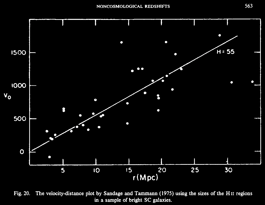 |
Non-CH
consistent clustering of redshifts around
certain periodic values. 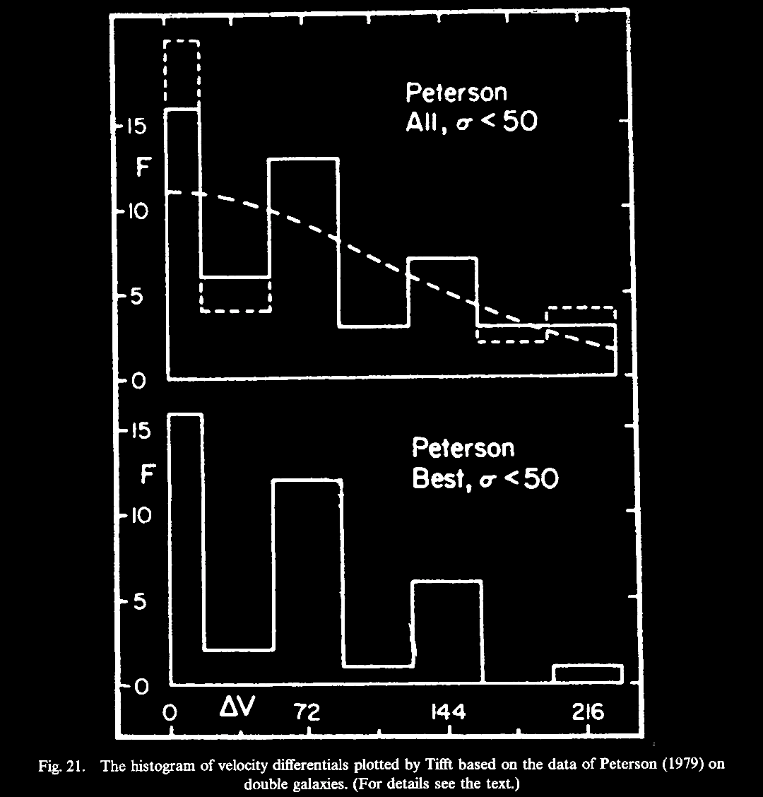 |
 |
 |
 |
These
following images, cited in the review, are not
the astronomical images in their original
quality. For the original, higher quality
images, see the original publications cited in
Prof. Narlikar's review. 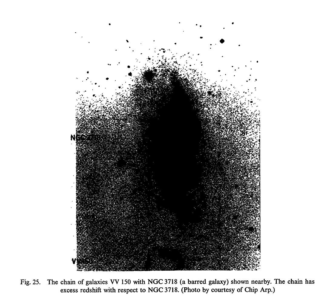 |
 |
 |
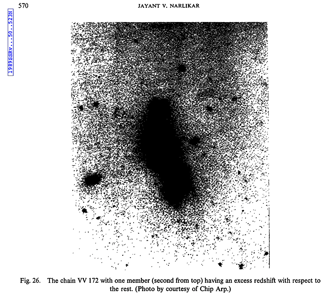
Companion
galaxies exhibit consistently higher redshifts
than the main galaxies in these groups. Under
the CH this should be more randomized. 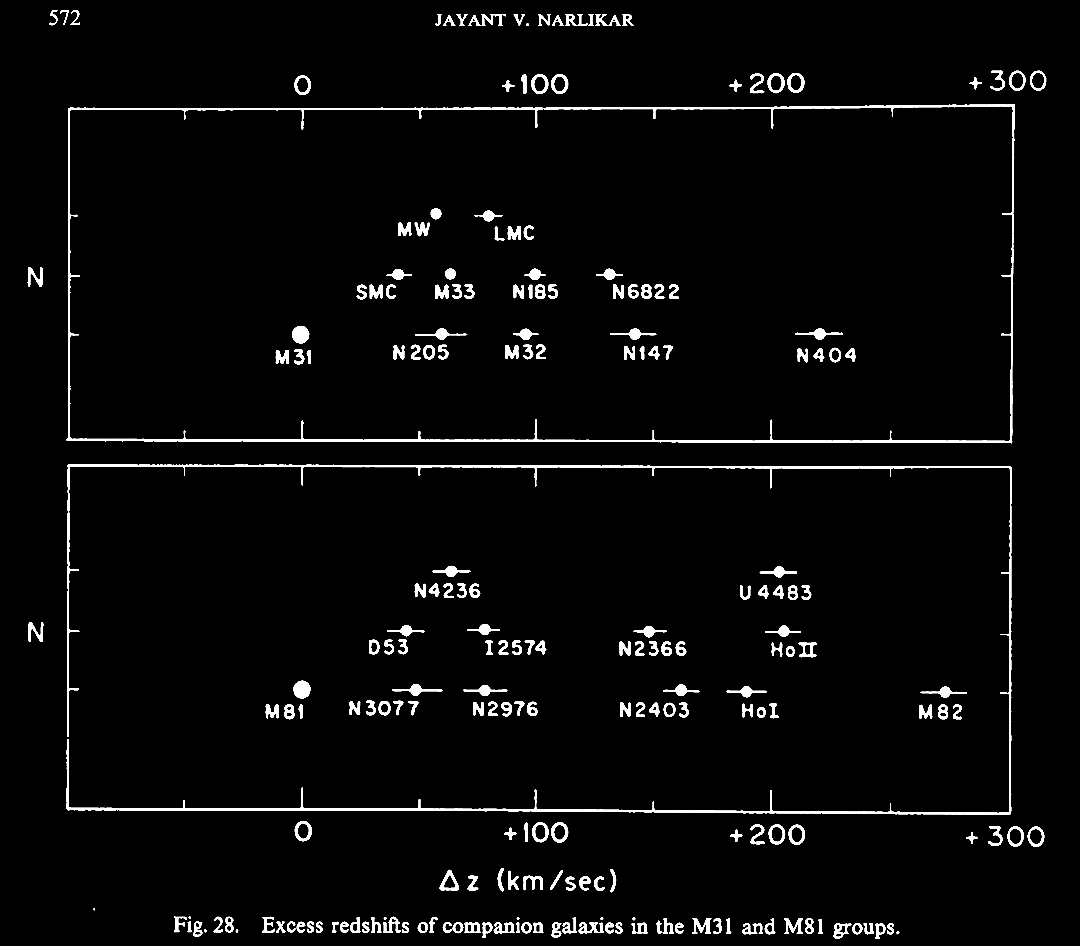 |
 |
 |
 |
 |
 |
 |
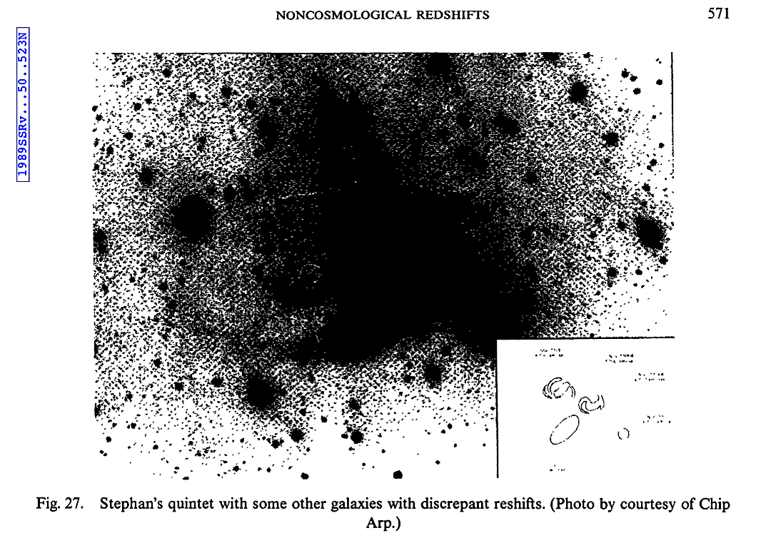
Under
the CH, QSOs should be randomly positioned in
the background, however they exhibit excess
clustering around near, bright galaxies. 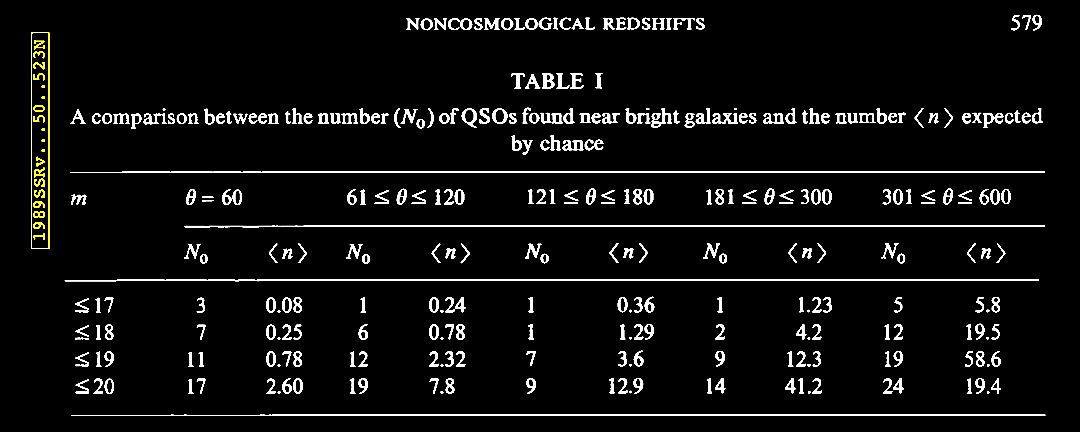 |
 |
Under
CH, there should be no such correlation. |
Juxtaposition
of higher redshift QSOs along the axis of NGC
3384, as if ejected along that axis. Under CH,
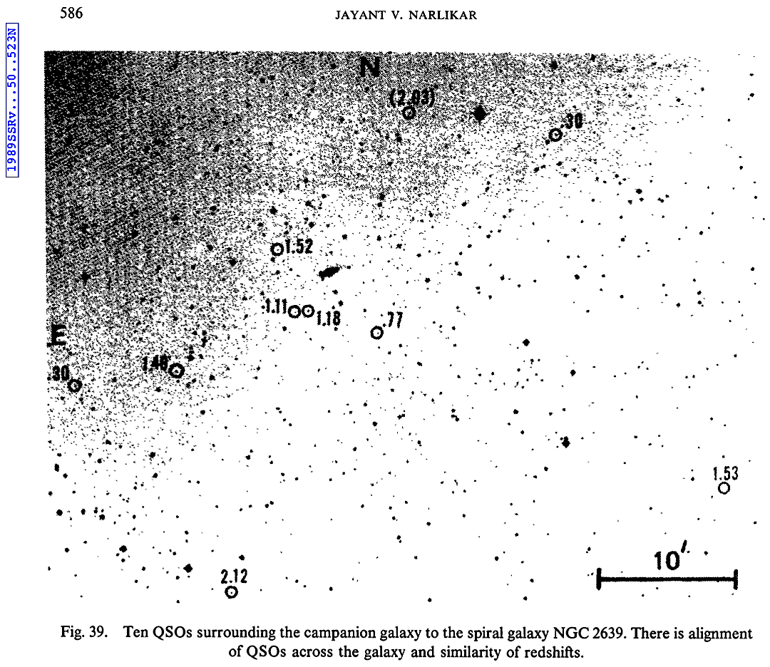
we would expect random background juxtaposition.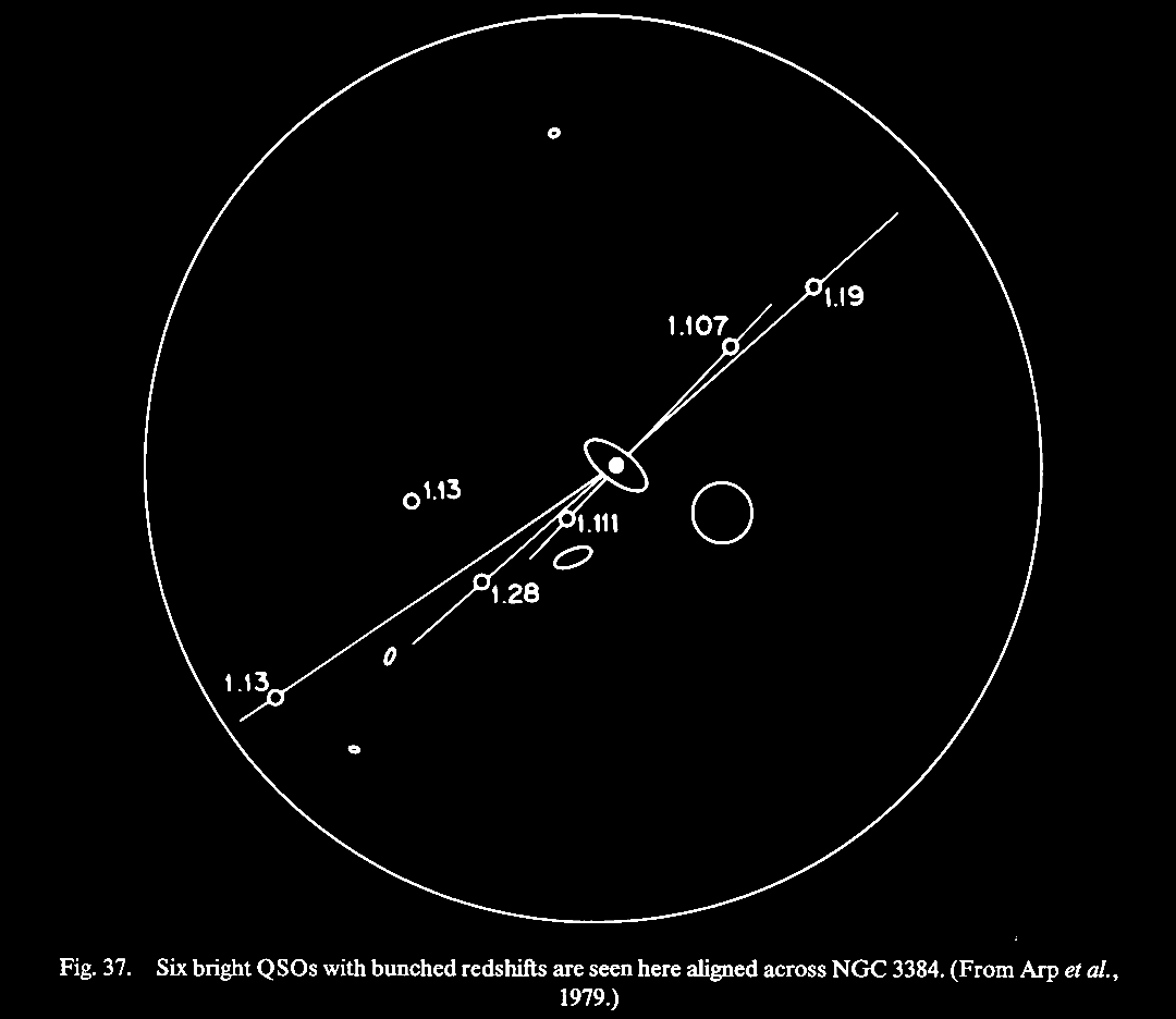 |
Although
the quality of this image is poor, the three
QSOs are juxtaposed with the spiral arms, and
exhibit location of their z values at
Karlsson peaks. 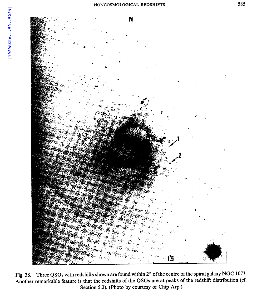 See larger version above as well: (Arrows added to image from http://www.astronomy.com/asy/default.aspx?c=a&id=3430). |
 |
AGN
galaxy M82, we now know, not only has the 4
juxtaposed higher redshift QSOs but up to 15 as
discussed in chapter IX. Vast Jets,
juxtapositioning referenced in chapter V. JWST v ΛCDM.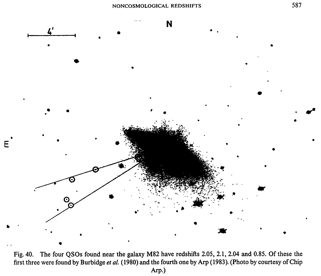 |
 |
 |
According
to the CH view of redshifts, these galaxies are
this discordant in size.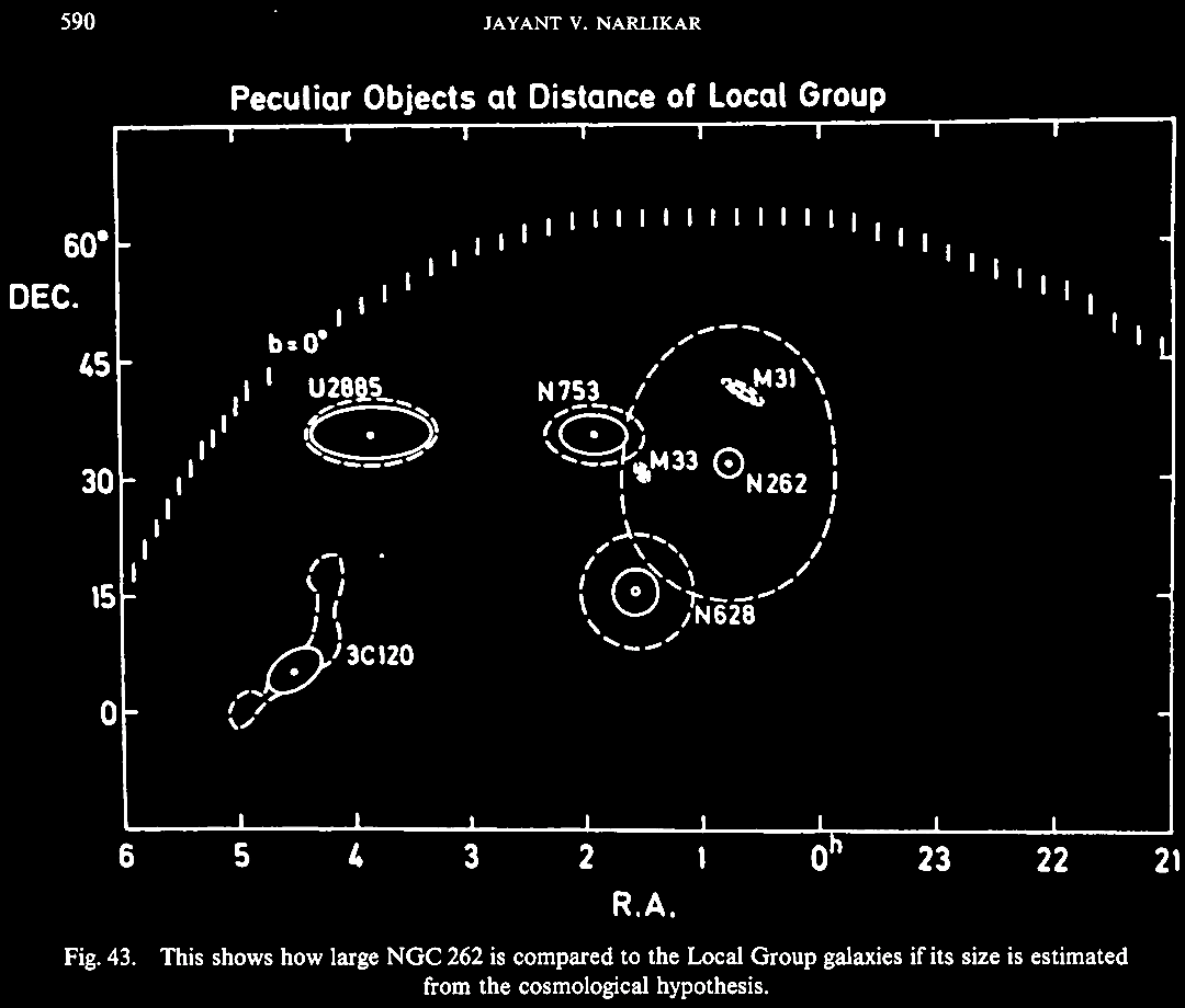 |
Redshift
values weirdly in excess with certain galactic
morphologies, namly S0 and Sbc and Sc.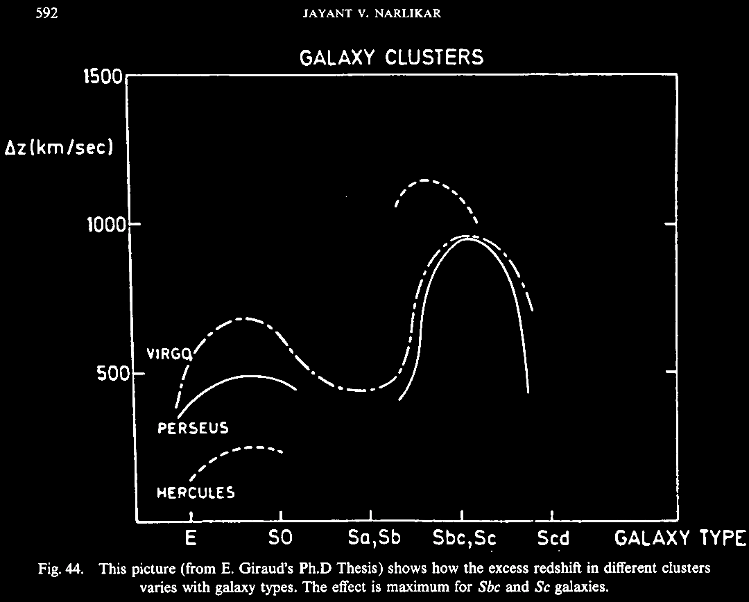 |
 |
In
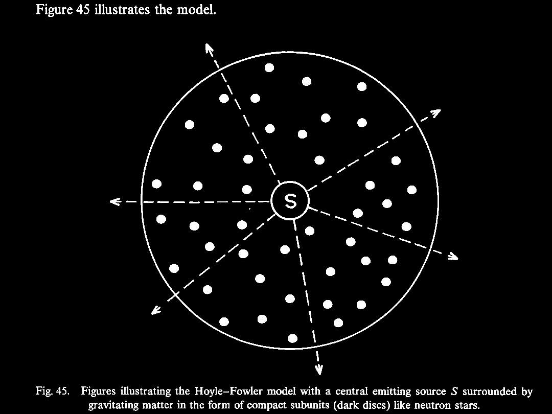
the HN Machian gravity-cosmology, less massive
particles closer to their origin are more highly
redshifted.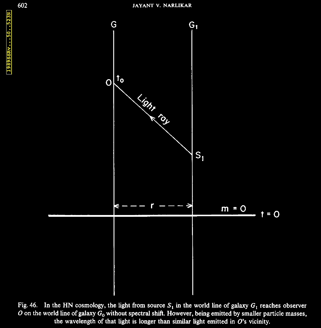 |
 |
 |
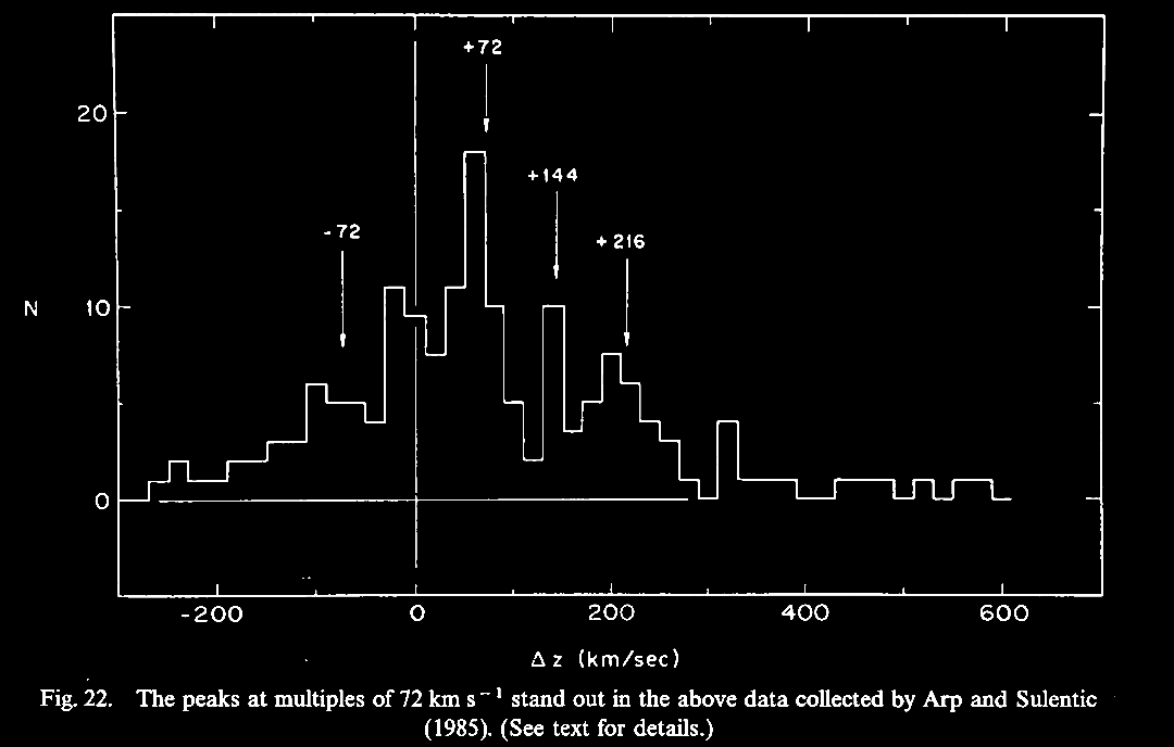
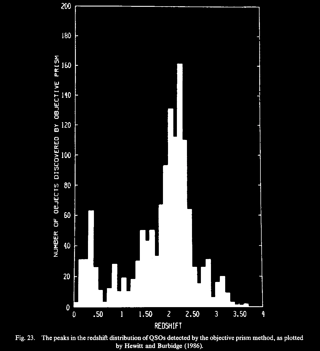
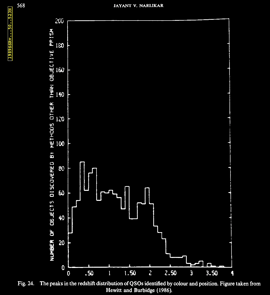
 Narlikar (1989).
We note that the empirical preferential clustering of redshifts around certain values began to be observed after 1970, and these were noted in the Narlikar review (1989) just cited.
Modified from figure 8-4 in H. Arp, 1998. Seeing
Red: Redshifts, Cosmology, and Academic Science.
Montreal, Quebec, Canada: Apeiron Press.
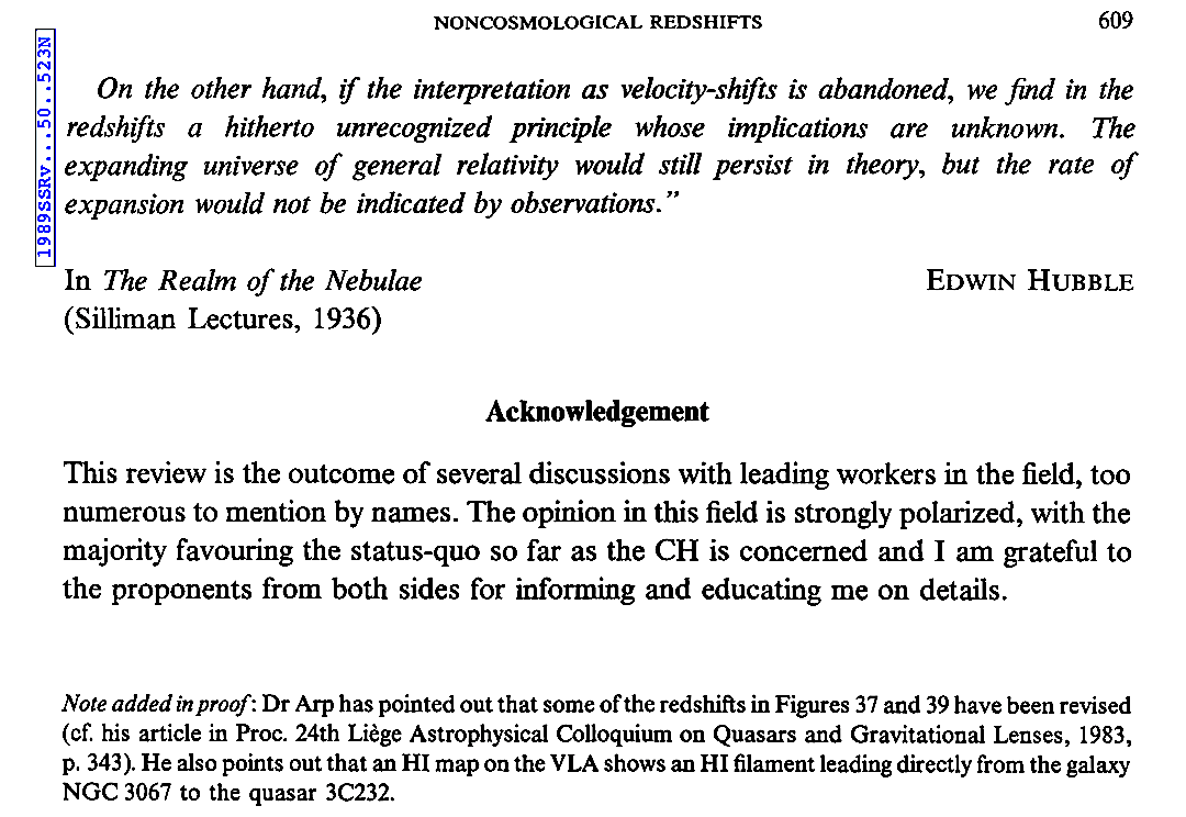
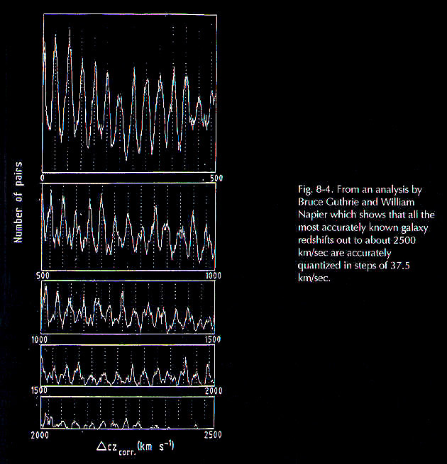
Representation of preferential clustering of redshift values (cited Arp, 1998) showing a preferential clustering around increments of 37.5 km s–1. In the case of QSOs / BSOs, a possible empirical relation which was pointed out early is 1 + z0 = (1 + zg)(1 + ze)(1 + zi), where z0 is the observed redshift, zg is the Doppler shift of the parent galaxy, ze is the QSO's Doppler shift (+ or -) from its putative ejection from the parent galaxy, and zi is an intrinsic redshift component-associated Machian age-mass scale in a matter creation process (Burbidge et al. 1999). That is one of the models of galactic cosmogony we will explore further.
Power spectrum of the redshifts of
97 spiral galaxies (Guthrie
& Napier, 1996; cit. in Hoyle et
al. 2000. A Different Approach to Cosmology: From
a Static Universe through the Big Bang Towards Reality.
Cambridge, UK: Cambridge University Press).
Frequencies of the redshifts of all
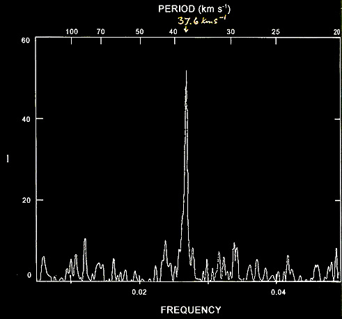
7315 then known QSOs with
peaks at z ~ 0.3, 1.4, 1.9-2.0. From Hoyle et al.
2000. A Different Approach to Cosmology: From a Static
Universe through the Big Bang Towards Reality.
Cambridge, UK: Cambridge University Press).
In 2003, a volume was published to
honor the late Sir Fred Hoyle (1915-2001) by C.
Wickramasinghe, G. Burbidge, & J. Narlikar. (eds.). 2003. Fred Hoyle's Universe. Dordrecht, The
Netherlands: Kluwer Academic Publishers, with lots of
invited scientists, astronomers, and astrophysicists, on
subjects as varied as Hoyle's contributions to people's
personal reminiscences, stellar structures and
evolution, cosmology, interstellar matter, and
panspermia. Among the chapters, two were
devoted to redshift periodicities: W. M. Napier on p. 139,
republished from A statistical evaluation of anomalous
redshifts. Astrophysics and Space Science 285
(2), 419.
https://doi.org/10.1023/A:1025452813441.
The
hypotheses Napier tested statistically were observations in
the light of so-called class of 'anomalous' redshifts for
pairs of galaxies and QSOs with widely different z-values,
often displaying bridges of luminosity between them. These tests are
critical tests of the universality of the Hubble distance
relation and whether the HBBC fails the test.
(a)
The first claim was that in the galactocentric frame of
reference, the Virgo cluster spiral galaxies have a
distribution with a periodicity of 71 km s–1,
which is similar to an early claim of 72 km s–1
in the Coma cluster of galaxies by
Tifft, W. C. 1976. Discrete states of
redshift and galaxy dynamics. I.
Internal motions in single galaxies. ApJ
206, 308. https://ui.adsabs.harvard.edu/abs/1976.
Napier (2003) figure 1 shows part of the
periodicty / redshift frequency data.
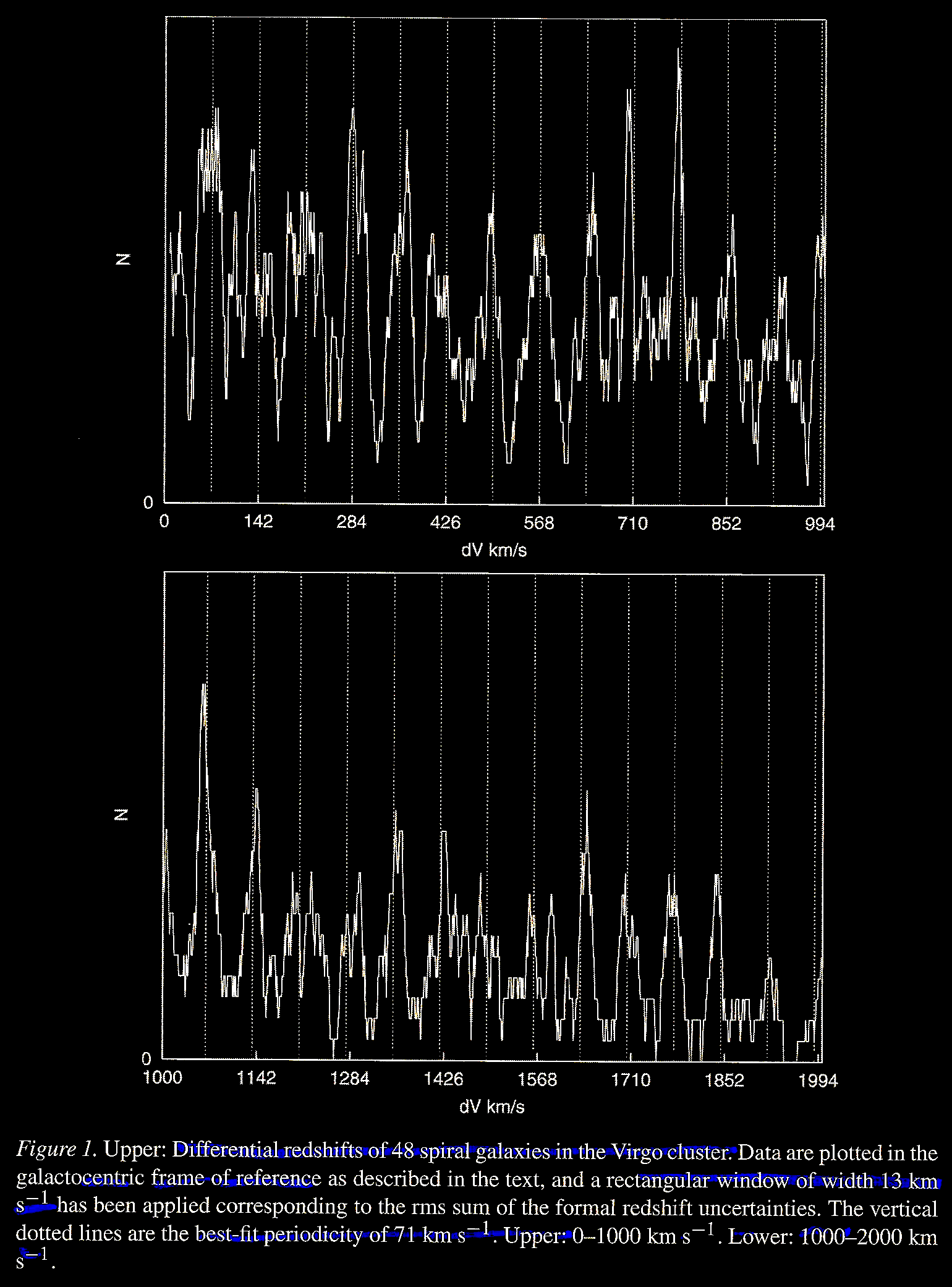
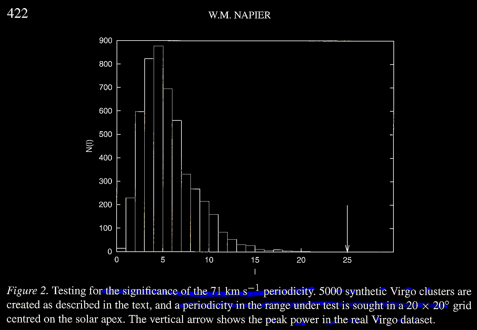
The significance of
the 71 km s–1,
periodicity was determined by synthetic
simulations of Virgo clusters. The statistical
tests were searches of 3-d spaces to find a
single Imax, that is, the
highest power to be found anywhere in the
parameter space of the study. The test results
for the real data set of the actual Virgo
Cluster are very robust indeed (Napier, 2003;
Figure 2).
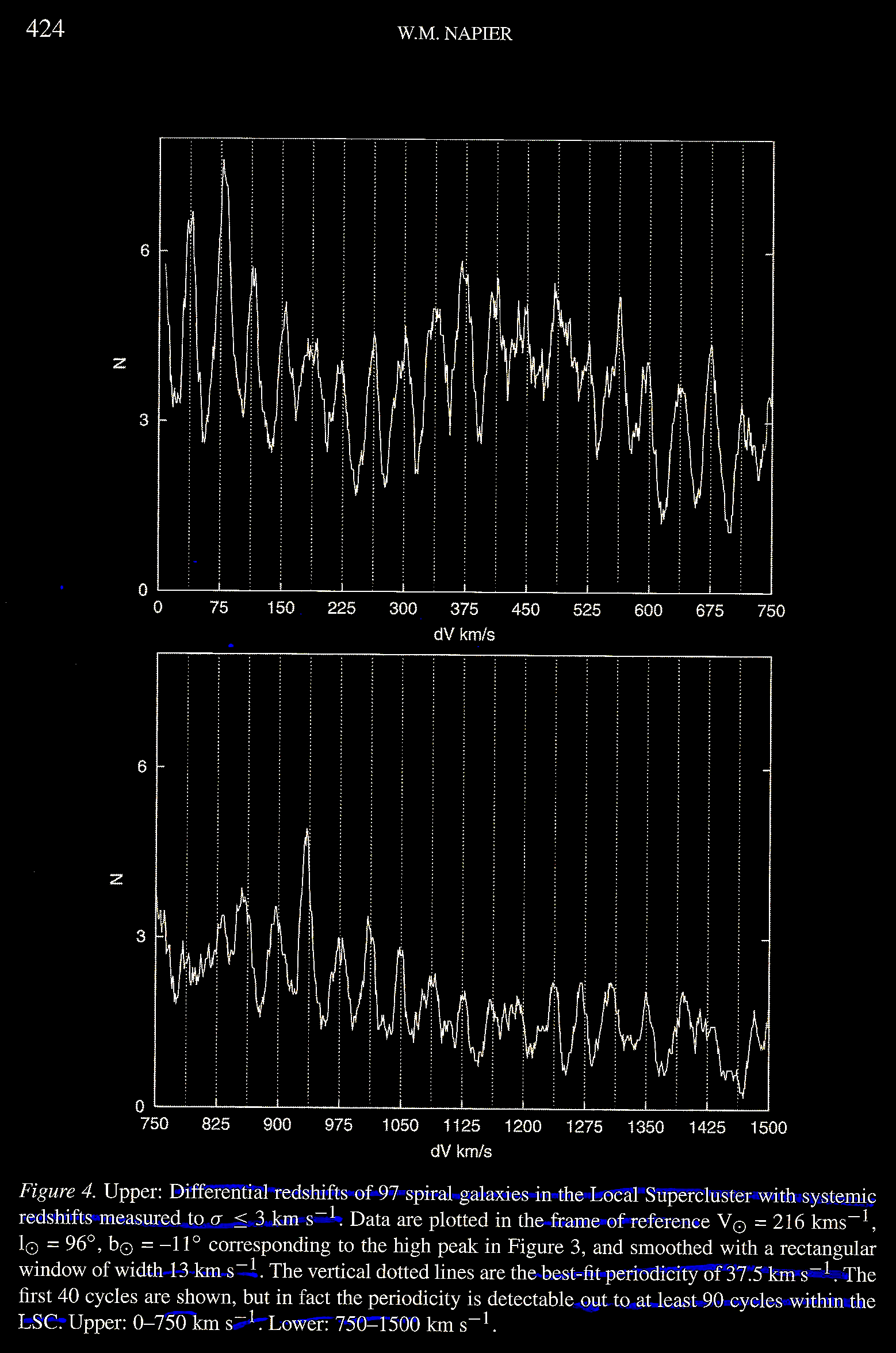
(b) The second claim was that
there is a galactocentric periodicity among
"wide-profile field [spiral] galaxies" of 36 km s–1
in the Local Super Cluster (LSC) as reported by Tifft
& Cocke. 1984. Properties of the redshift. ApJ
287, 492. https://doi.org/10.1017/S0252921100005546.
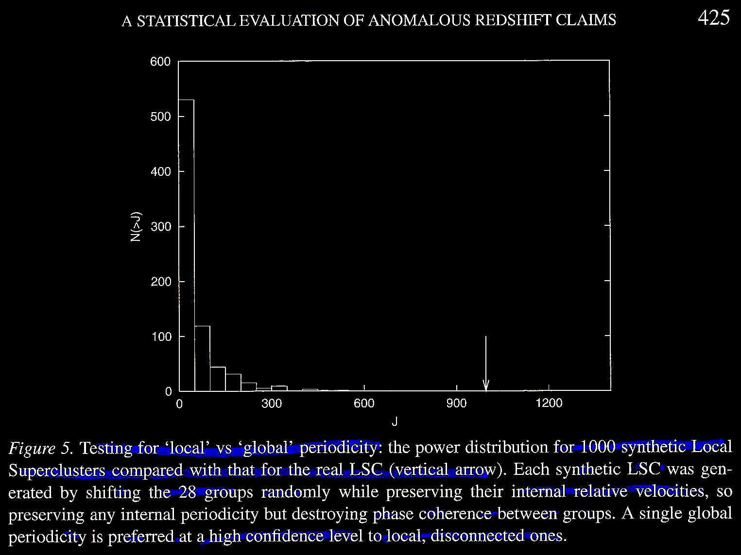
Napier's more accurate tests showed a 37.5 km s–1 periodicity in the LSC, as
portrayed in Napier, Fig. 3.
And in Figure 4,
which shows a persisting and robust 37.5 km s–1
periodicity out to 40 cycles, but detectable out to at least
90 cycles, Napier found. This is shown by Arp in 1998 as
indicated above, including by a power spectrum test (see
figure cited by Hoyle et al. 2000 on the power
spectrum of a periodicity of 37.6 km s–1).
As Tifft and Cocke (1984) had
suggested, a robust 37.5 km s–1 redshift
periodicity, in a galactocentric frame of reference, has
been found within the Local Super Cluster (LSC). A J
statistical test with simulations for artificial LSCs
was used to test whether the periodicity is a local or a
global effect.
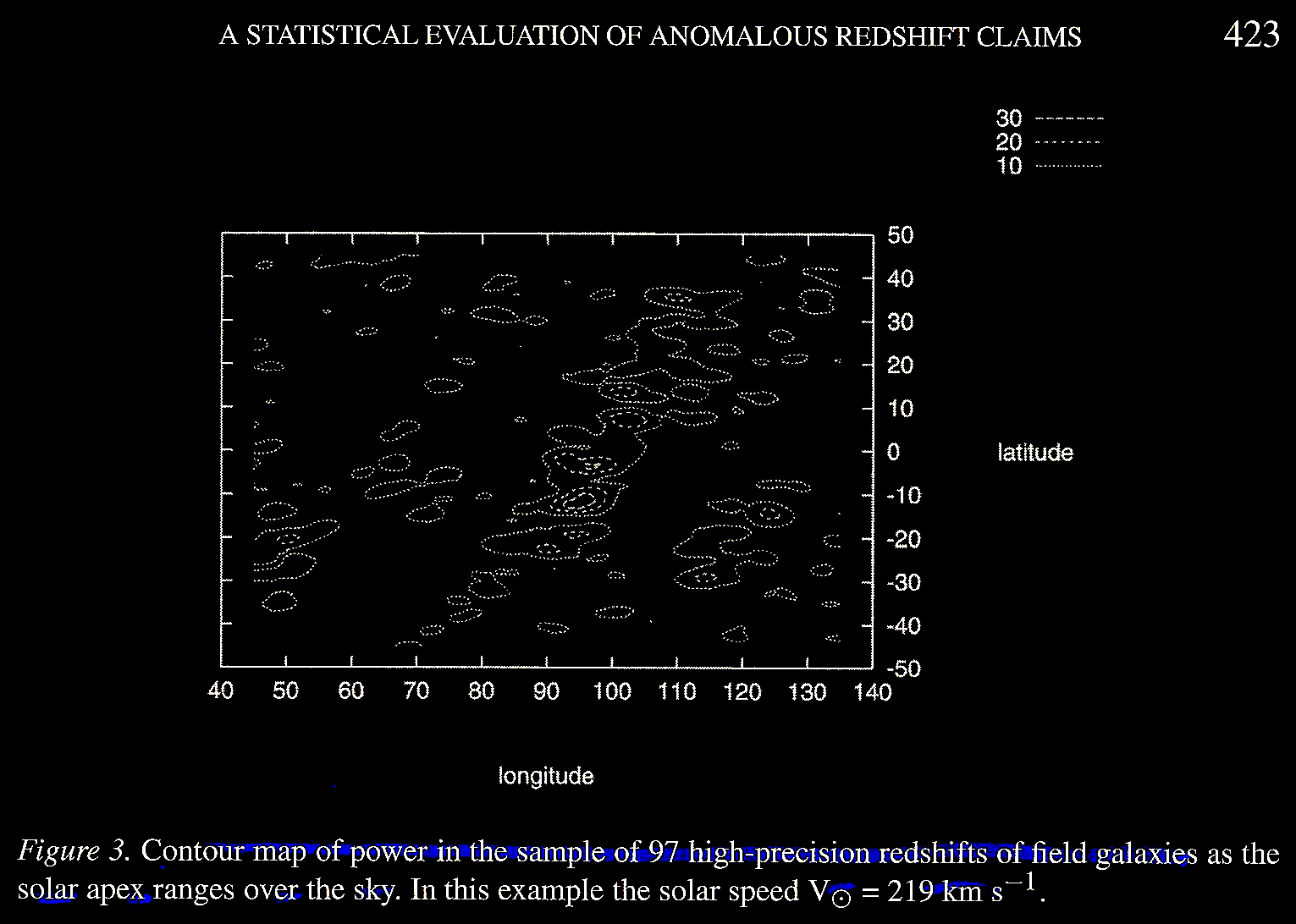
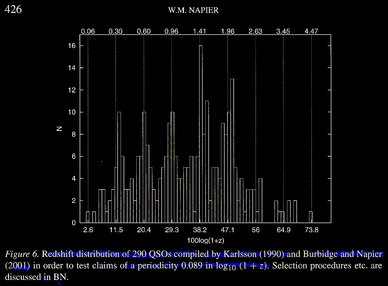
(c) The third claim was that quasars or QSOs clustered around bright local galaxies exhibit a redshift periodicity of 0.89 in log10 (1 + z), although it is not clear whether this is within the galactocentric frame of reference or local periodicities from discrete velocity residuals with respect to the variable solar apex used in assessing the periodicity found in the study of the Virgo Cluster done by Guthrie, B. N. G. & Napier, W. M. 1991. Evidence for redshift periodicity in nearby field galaxies, MNRAS 253 (3), 533. https://doi.org/10.1093/mnras/253.3.533. See also Napier, 1999. Quantized redshifts - New physics or old muddle? Symposium - International Astronomical Union, Volume 194: Activity in Galaxies and Related Phenomena, pp. 290-294. https://doi.org/10.1017/S0074180900162126. What they found was that there is indeed such a periodicity in the distribution of the QSOs appearing around local galaxies.
The
work of Karlsson (1990. Astronom. Astrophys. 239,
50) and and that of Burbidge & Napier, 2001; The
distribution of redshifts in new samples of quasi-stellar
objects. Astrophys. J. 121 (1), 21. https://doi.org/10.1086/318018,
was confirmed.
Napier concluded that if all of the above periodicities (a), (b),and (c) are real, then they must be the effects of some single underlying phenomenon and must be connected with the linearity of the local Hubble flow. Again, a cosmology other than the standard HBBC was indicated. We will return to this Burbidge & Napier (2001) paper below, after discussion of Tifft's modeling.
Another paper from the same memorial
volume for Fred Hoyle was Tifft, W. 2003. Redshift
periodicities, the galaxy-quasar connection. Astrophysics
and Space Science 285 (2), 429. https://doi.org/10.1023/A:1025457030279.
This paper develops the consequences of a particular
decay model for predicting the periodicities in redshift
found in various data sets, including the Hubbled Deep
Field (HDF) and Hubble Southern Deep Field (SDF),
tackling three classes of observations of intrinsic
redshifts departing from the linear Hubble redshift
relation, (α) characteristic peaks in QSO redshift
distributions, (β) associated objects with very
discordant redshifts, and (γ) normal galaxy redshift
quantization.
Tifft
(2003) Figure 1 illustrates the periodic quantized redshift
distribution for double glaxies (Tifft & Cocke, 1989).
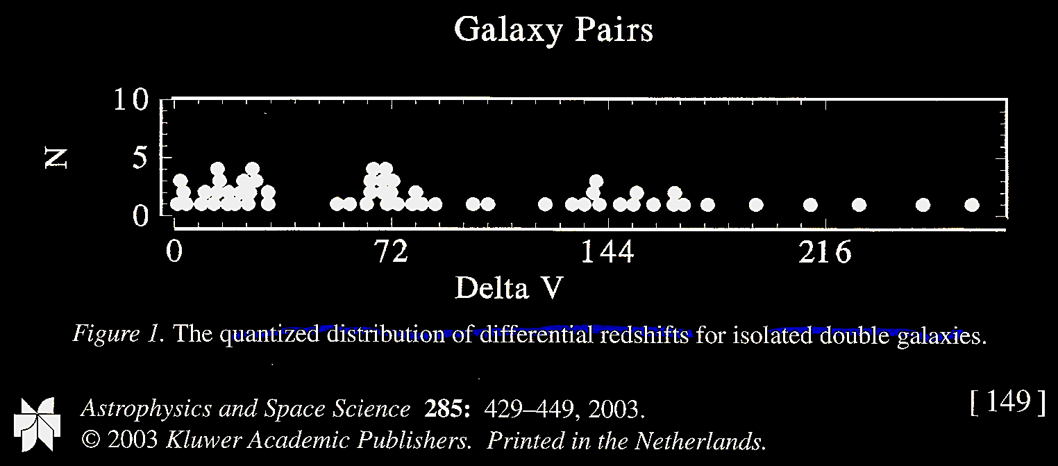
Figure 2 shows the characteristic redshift
periods observed globally using concepts which predict the
discrete values (Tifft, 1996).
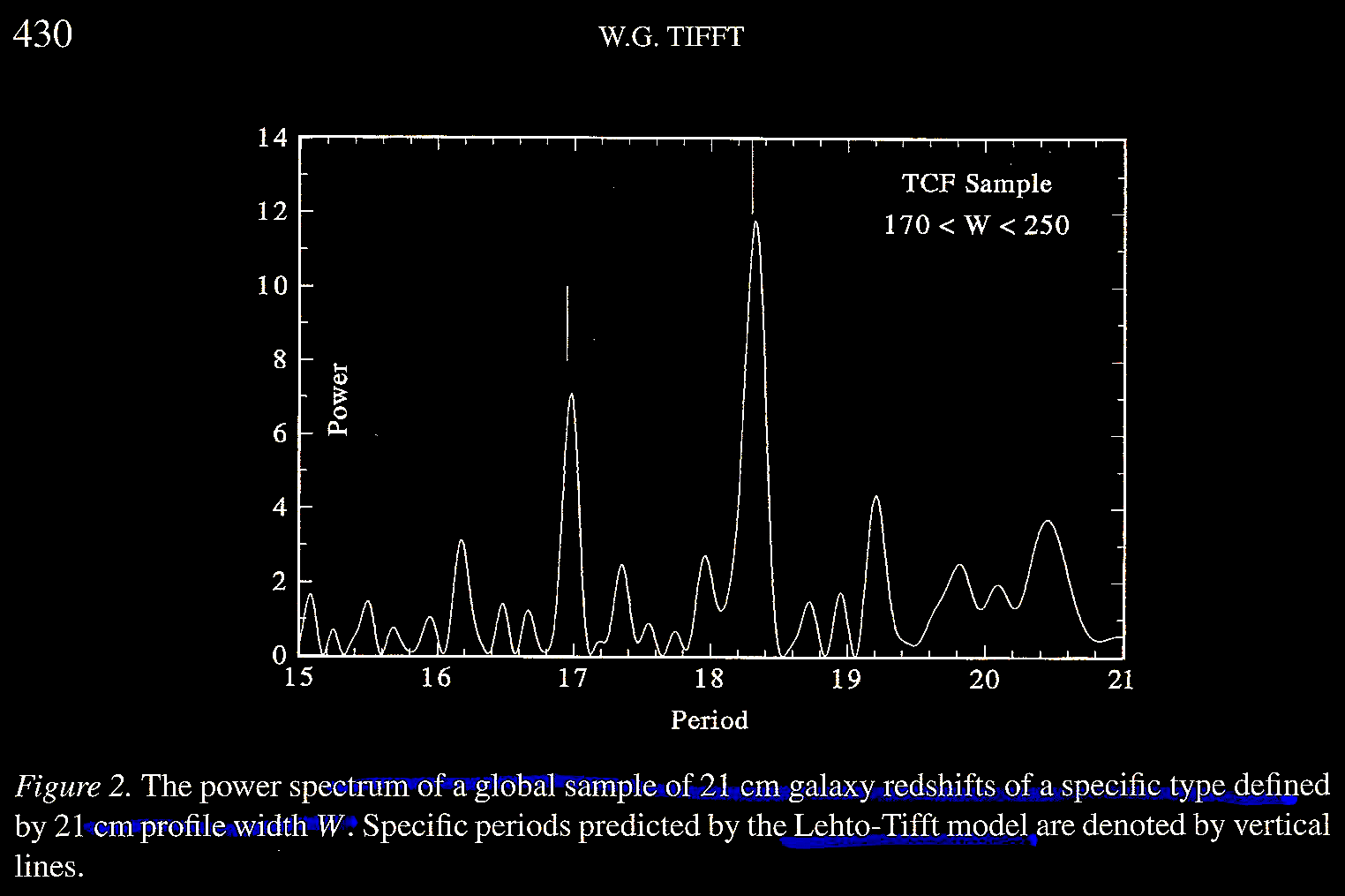
A first principles Planck
decay process & the Lehto-Tifft quantization model
equations. Although previous work (before 1992)
had focused on empirical periodic intervals observed
differentially or globally in a galactocentric frame of
reference, the emphasis shifted thereafter to the cosmic
background frame of reference. Finnish physicist Ari
Lehto put forward a mechanism for predicting
redshift periodicities (1990. Chinese J. Phys. 28,
15), which Tifft (1996; 1997) tested, confirmed, and
developed into the Lehto-Tifft quantization model with a
set of equations: Tifft, W. G. 1996. Global redshift
periodicities and periodicity structure. ApJ 468,
491. http://dx.doi.org/10.1086/177710;
and Tifft, 1997. Global redshift periodicities and
variablility. ApJ 485, 465. https://iopscience.iop.org/article/10.1086/304443.
In what follows, we closely follow Tifft (2003):
Lehto
(1990) planned to describe fundamental particle properties
using first principles, namely beginning with the original
Planck units of Max himself (link),
listed here with their modern values all calculated using 3
fundamental constants in modern values, the velocity of
light in vacuo, or c = 2.99792458 x 10⁸
m s–1
(link),
the reduced (divided by 2π, i.e., it's Dirac formulation)
Planck constant ħ = 6.582119569 x 10⁻¹⁶
eV⋅s (link),
and the gravitational constant G = 6.674 x 10⁻¹¹ m3⋅kg–1⋅s–2 (link):
- the Planck
time (T) = 5.391247(60) x 10–44 s,
- the Planck
length (L) = 1.616255(18) x 10–35 m,
- the Planck
mass (M) = 2.176434(24) x 10–8 kg,
- and the
Planck temperature (Θ) = 1.416784(16) x 1032
K, as well as we should add
for reasons later to be apparent,
- the coherently derived Planck unit of the Planck energy (L2MT–2) = 1.2209 x 10¹⁹ eV, converted from joules to electron volts, also for reasons later to be apparent.
where N is an integer ≥ 0. In applying this to particle physics, we replace c with the Planck mass (M) or energy (L2MT-2). The above equation is significant in being a general form comparable to Kepler's Third Law in ordinary space, where "a spatial distance relates to the 2/3 power of a time interval,... a unique property of 3-d spaces." This suggests "the possibility that temporal/frequency/energy space is actually 3-dimensional." If such a "3-d temporal space" flows relative to a "3-d spatial space" then the constancy of c and the applicability of special relativity are preserved. "Temporal space" is quantized into a stepwise decay process from the fixed units indicated. In a dynamic 4-space with 3-space and flowing 1-time, there are no such restrictions, so according to Tifft (2003), quantum physics and continuous, infinitesimal classical physics can co-exist.
At this point, Tifft argued that one may re-write equation (1) to distinguish cube-root doubling families thus
where D is the number of doublings and L = 0, 1, 2 to specify which root is utilized. Tifft (2003) points out that equation (2) predicts most redshift periodicities, however to account for all of the observed periodicities, one needs a second cube root to produce 9 9th-root famliies distinguished by a n index T:
Equation
(3), claims Tifft (2003), "completely and uniquely
describes" all of the periodicities observed as of Tifft
(1996, 1997). The index T values are not random, but
involve pure doubling, T = L = 0, the
dominant relation, followed by a 'Keplerian' T = 6 (L
= 2) value, where the odd T values are shifted by 1
as in T = 1, 5, 7 which is less common, and
finally the even values of T = 2, 4, 8 are rare or
absent entirely. Weirdly, which T family is observed
seems to relate to galaxy morphology (Tifft, 1997). Equation
(3) seems to describe redshift distributions in local
galaxies, whereas at higher redshifts and deeper in space,
the T = 0 family "becomes increasingly dominant."
A
correction must be made to assess underlying redshift
quantization, and that is, redshift intervals "dilate with
distance" because of effects both relativistic and
geometric, which must be removed. Classically in cosmology,
'curvature' is described by the 'deceleration' parameter q0,
while the Hubble 'constant' serves as a function of time, H
= H(t) = f(z, q0),
which in a flat or Euclidean cosmos would have q0
= 1/2. Removing the z-dependent distortion
is called the 'cosmological' correction in redshift. Tifft
& Cocke (1984) investigated the 'cosmological'
correction for global redshift quantization studies. Tifft
(1996) assumed that redshift intervals dilate as √[H(t)]
to show a linearization of galaxy redshifts out to
>10,000 km s–1 provided that q0
= 1/2. Tifft (2003), whose treatment we are following,
showed that this correction works well out to z = 1
or 2, far enough to encompass, as we shall see, the Hubble
Deep Fields North and South, taken in the 1990s. Following
the classical H(t) formulation to find the
function H(t)
= f(z, q0), Tifft
integrated with a Taylor expansion around q0 =
1/2 to arrive at a closed relation between z(observed)
and z(Lehto-Tifft):
(4)
zobs = {[z(LT)/4]
+ 1}4 – 1
z(LT) = 4[(1 + zobs]1/4
– 1,
a formulation
empirically-fitting all of the then available data (Tifft,
1996, 1997). Tifft (2003) uses equation (4) to convert
observed redshift to z(LT)
to evaluate redshift quantization. Since equation
(4) is consistent with the "temporal 3-d space"
model discussed above, where energies vary with
temporal volumes as t3 so that
if photon redshifts are a result of energy
densities, which vary as these volumes evolve, the
rate of change will be observed as H = H(t) = f(z,
q0).
The spatial volume will evolve as t2 so
that H = H(t) = f(z,
q0)
depends on t2
redshift periodicities vary as √[H(t)]
exactly as observed.
At this point, let's look at the
data which Tifft (2003) summarized in light
of the doubling decay process postulated in
the Lehto-Tifft model:
Tifft's (2003) Table 1 shows that
the redshift peak locations match the
empirical logarithmic sequence of QSO
redshift peaks observed by Karlsson, K. G.
1977. On the existence of significant peaks
in the quasar redshift distribution. A&A
58 (1,2), 237. https://articles.adsabs.harvard.edu//full/1977.
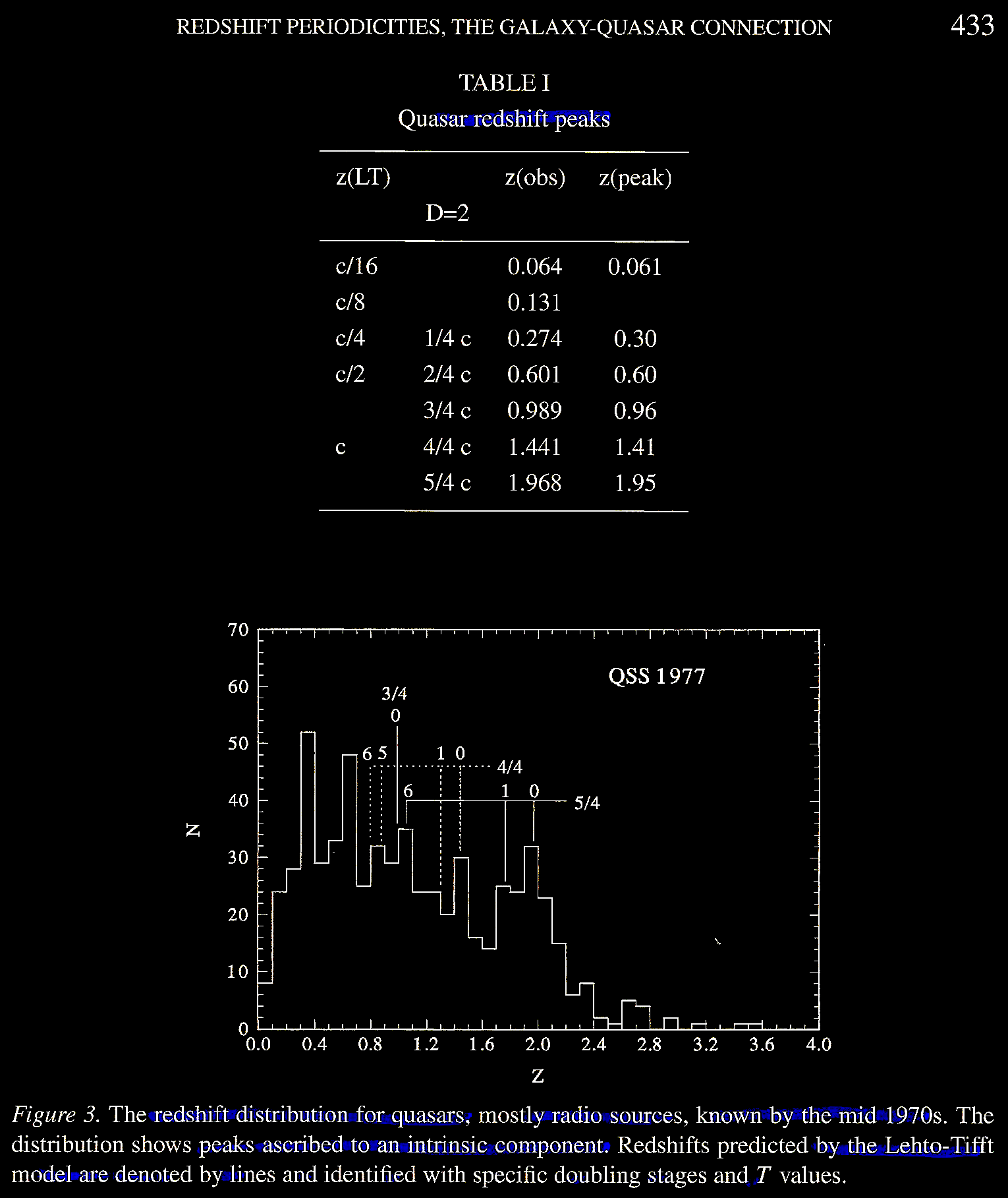
Tifft (2003) Figure 3 shows the quasars
known in 1977.
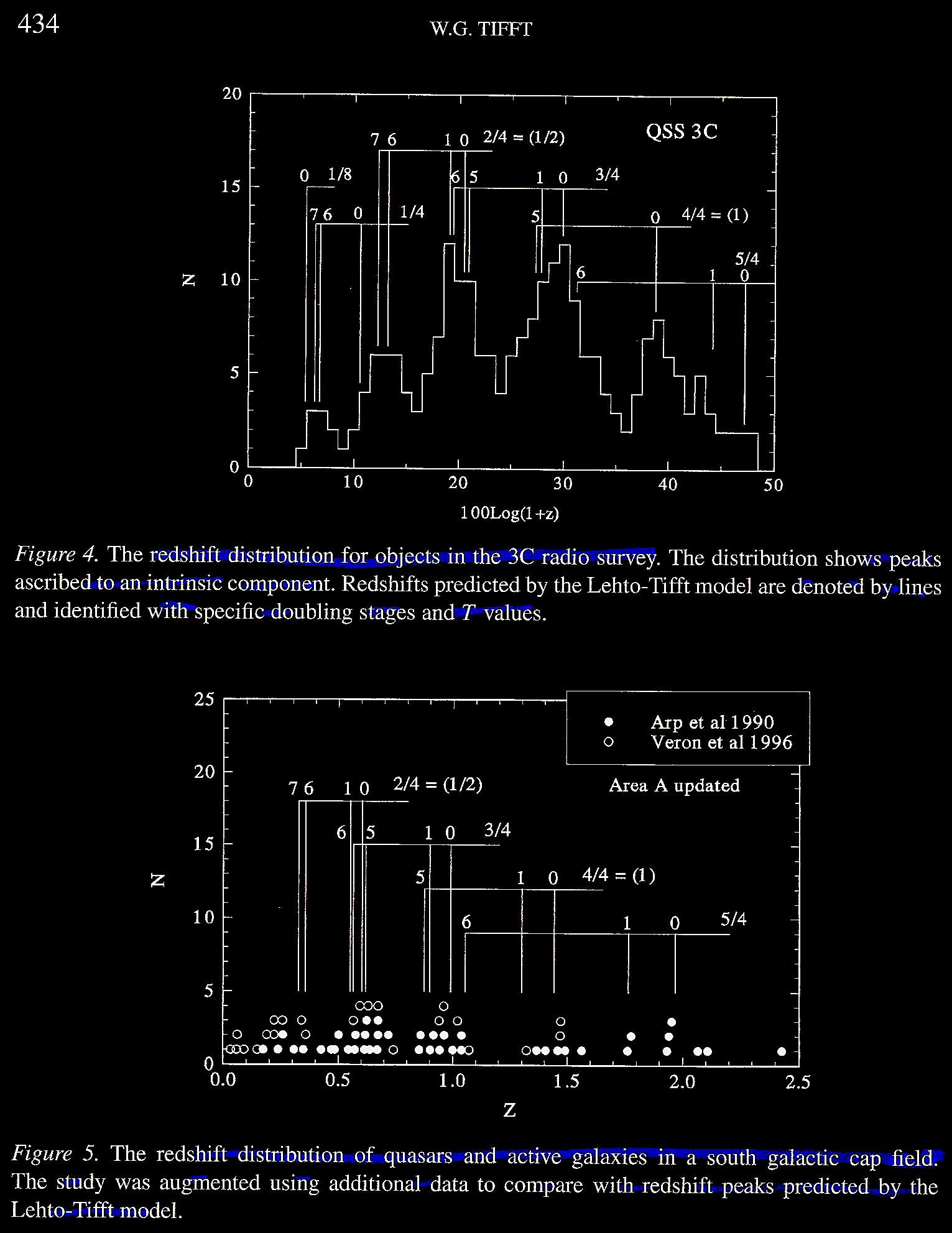
When one adds the full set of the
3rd Cambridge catalog of quasars, one gets
the results in Tifft (2003) Figure 4. In
addition, one can add the quasars from
studies referenced involving the "south
galactic cap field" in Tifft (2003) Figure
5, differentiated by filled and open
circles.
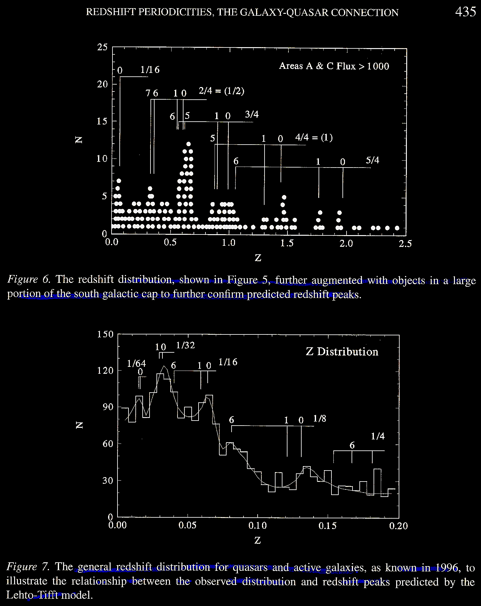
The Karlsson empirical peaks and
the Lehto-Tifft model-predicted peaks
continue to pile higher (Tifft, 2003, Fig.
6) when all of the data from the galactic
southern hemisphere south of the initial
field are included as found in the QSO and
active galaxy catalogue of Veron-Cetty &
Veron 1996. 7th ed. A Catalog of Quasars
and Active Galaxies. ESO Scientific
Report 17. See
https://heasarc.gsfc.nasa.gov/W3Browse/all/veroncat.html.
Tifft (2003) Figure 7
shows that there may be
a c/8 peak also.
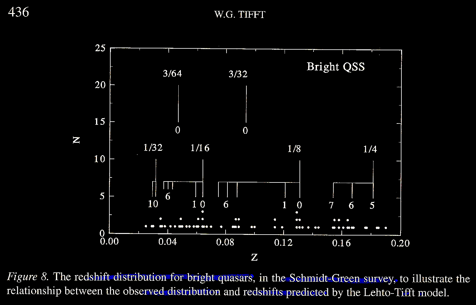
The trend is extended not on from
the c/8 region but also to the c/16
region of the graph when data from Schmidt,
M. & Green, R. F. 1983. Quasar evolution
derived from the Palomar bright quasar
survey and other complete quasar surveys. ApJ
269, 352. https://articles.adsabs.harvard.edu/full/1983ApJ,
as illustrated in Tifft (2003) Figure 8.
The Lehto-Tifft model suggests
that ongoing Planck unit decay would also
yield less active QSOs and ordinary
galaxies, thus linking galaxies and quasars.
Decay from the first doubling would show a c/2
associated with z = 0.6 quasar peak.
The redshift 'spectrum' would be T =
0 dominant, have various decay product
periodicities, and importantly, "discordant
redshift associations where physically
related objects have decayed into different,
but related states" as has been discussed by
Halton Arp and a few others for years.
Although local decay has gone to D =
12-16, but at z = 0.5, the model
predicts periodicities in D = 4-9,
i.e., c/16 - c/512 (20,000+
to 500 km s–1) range.
In 1995, the Hubble Space
Telescope made a deep and long exposure in a
small patch in the celestial northern
hemisphere called the Hubble Deep Field
(HDF), which provided opportunity to examine
redshifts of faint and distant galaxies.
-1995_15jan1996.jpg)
This hypothesis could be tested in
2003 with the Hubble Space Telescope (HST)
Hubble Deep Field (HDF) and Southern Deep
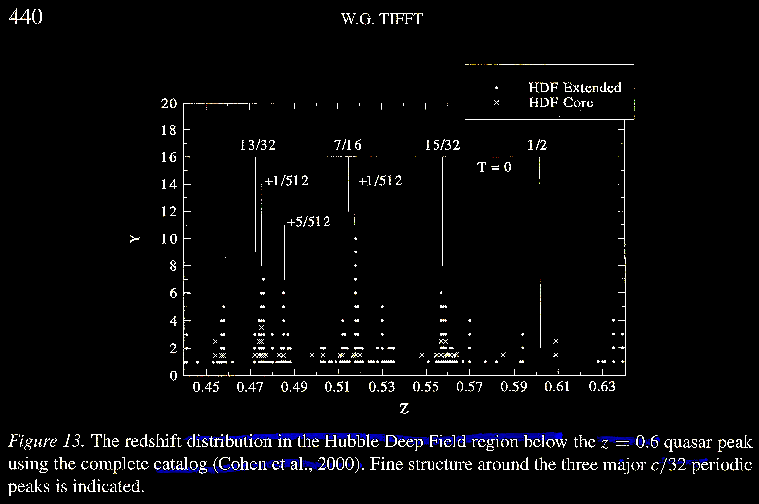
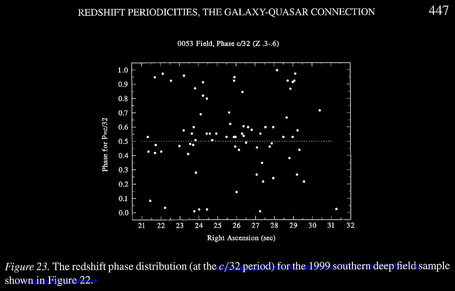
Field (SDF), in Tifft (2003) Figure 9, as
adapted from Cohen et al.
2000. Caltech faint galaxy redshift survey.
X. A redshift survey in the region of the
Hubble Deep Field north. ApJ 538
(1), 29. https://iopscience.iop.org/article/10.1086/309096/pdf.
.
.
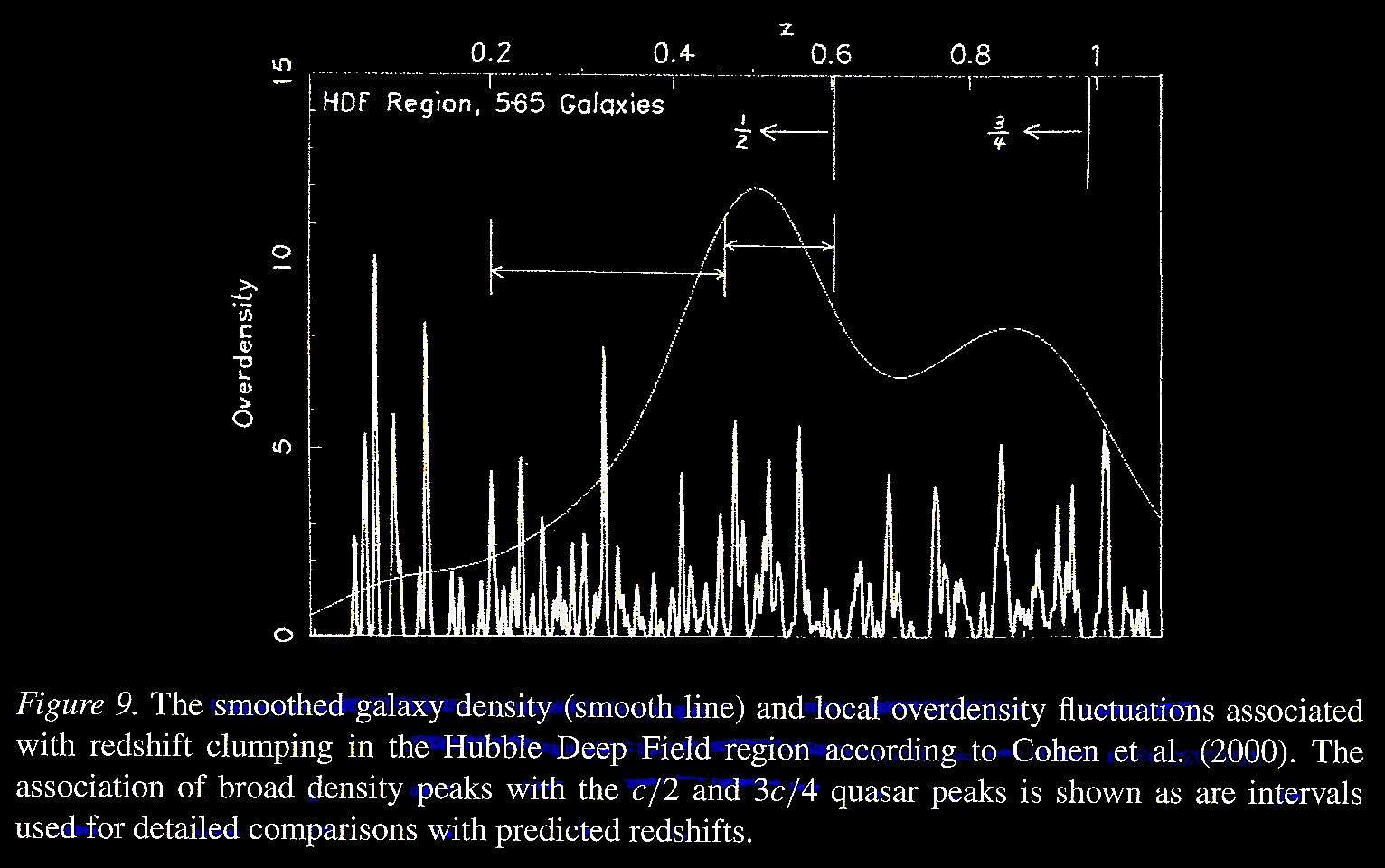
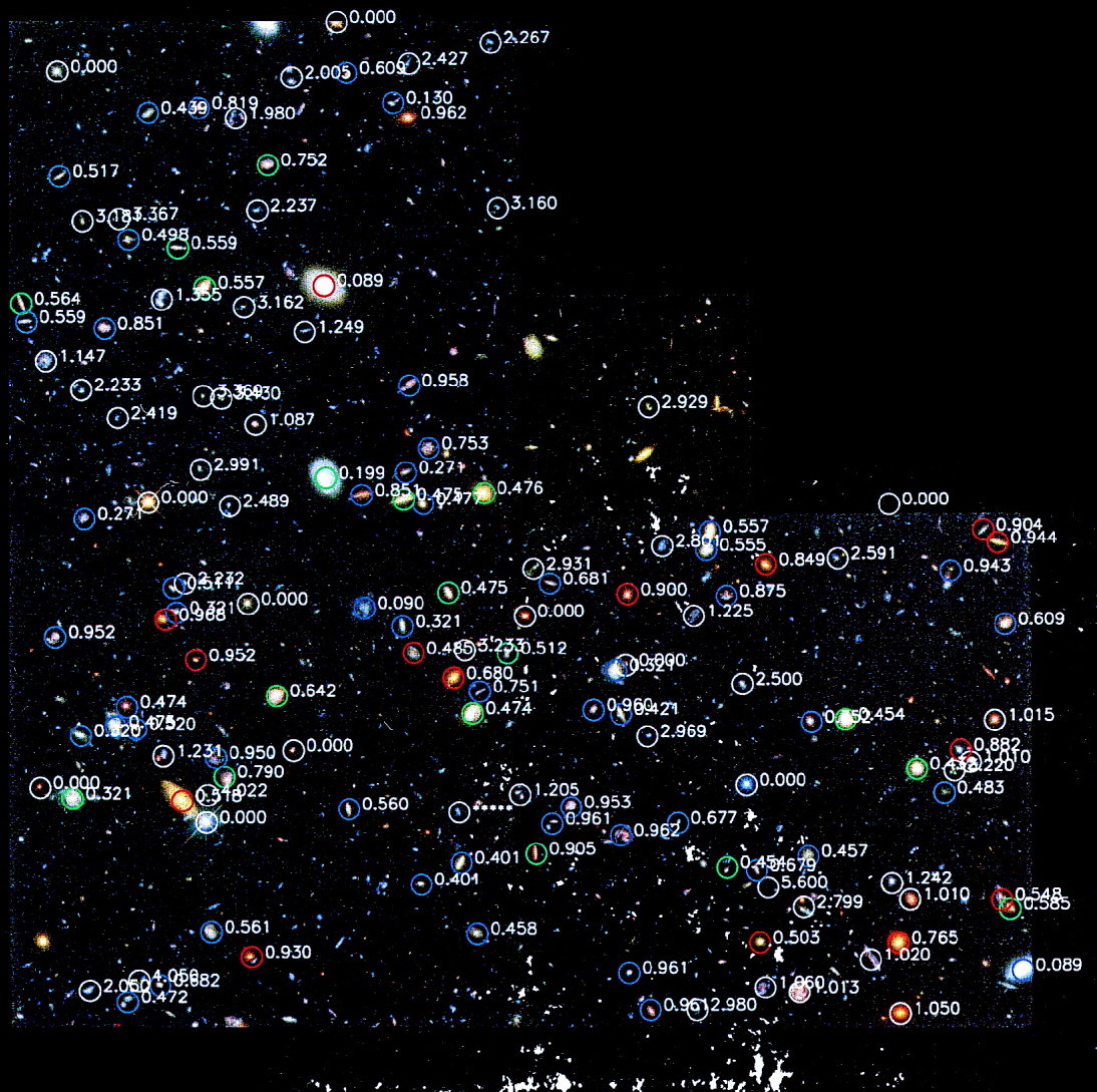
The following Figure 2 from Cohen et al. (2000) superimposes on the HDF the redshifts as well as their color-coded spectral classes, with circles of different colors for redshifts z ≤ 1 and white circles for redshifts z > 1. Cohen and colleagues classified galaxy spectral classes as including galaxies with dominant emission lines (ℰ), galaxies with dominant absorption lines (𝒜), galaxies with intermediate spectra (ℐ), and galaxies with broad emission lines (𝒬). The authors note that starburst galaxies with higher Balmer lines Starburst galaxies with higher Balmer emission lines (Hγ, Hδ, etc.) are classified (ℬ). However, the authors point out, "but for such faint objects, it was not always possible to distinguish them from 'ℰ' galaxies."

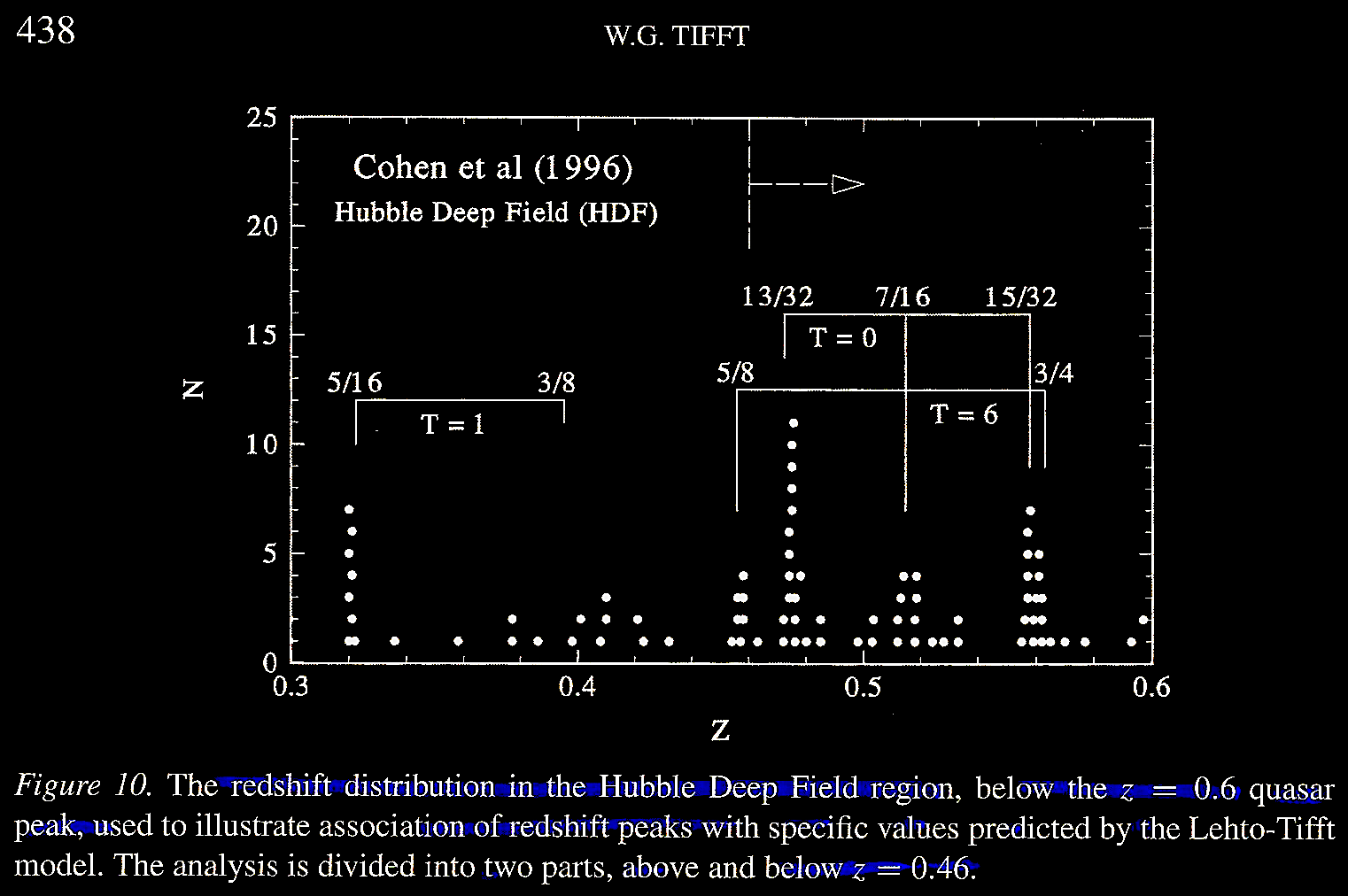
Tifft's first study (1997) used
the data from Cohen et ai. 1996.
Redshift clustering in the Hubble Deep
Field. ApJ 471 (1), L5. https://iopscience.iop.org/article/10.1086/310330.
That analysis is seen in Tifft (2003) Figure
10. The model predicted T = 1 and T
= 6 values are present, especially at the c/2,
c/16, and c/32 peaks.
Tifft (2003) Figure 11 showed how
precise is the fit to these three peaks, and
where the strongest peak was. However, a
larger sample was needed and became
available with Cohen et al. (2000)
as illustrated in Tifft (2003) Figure
12.
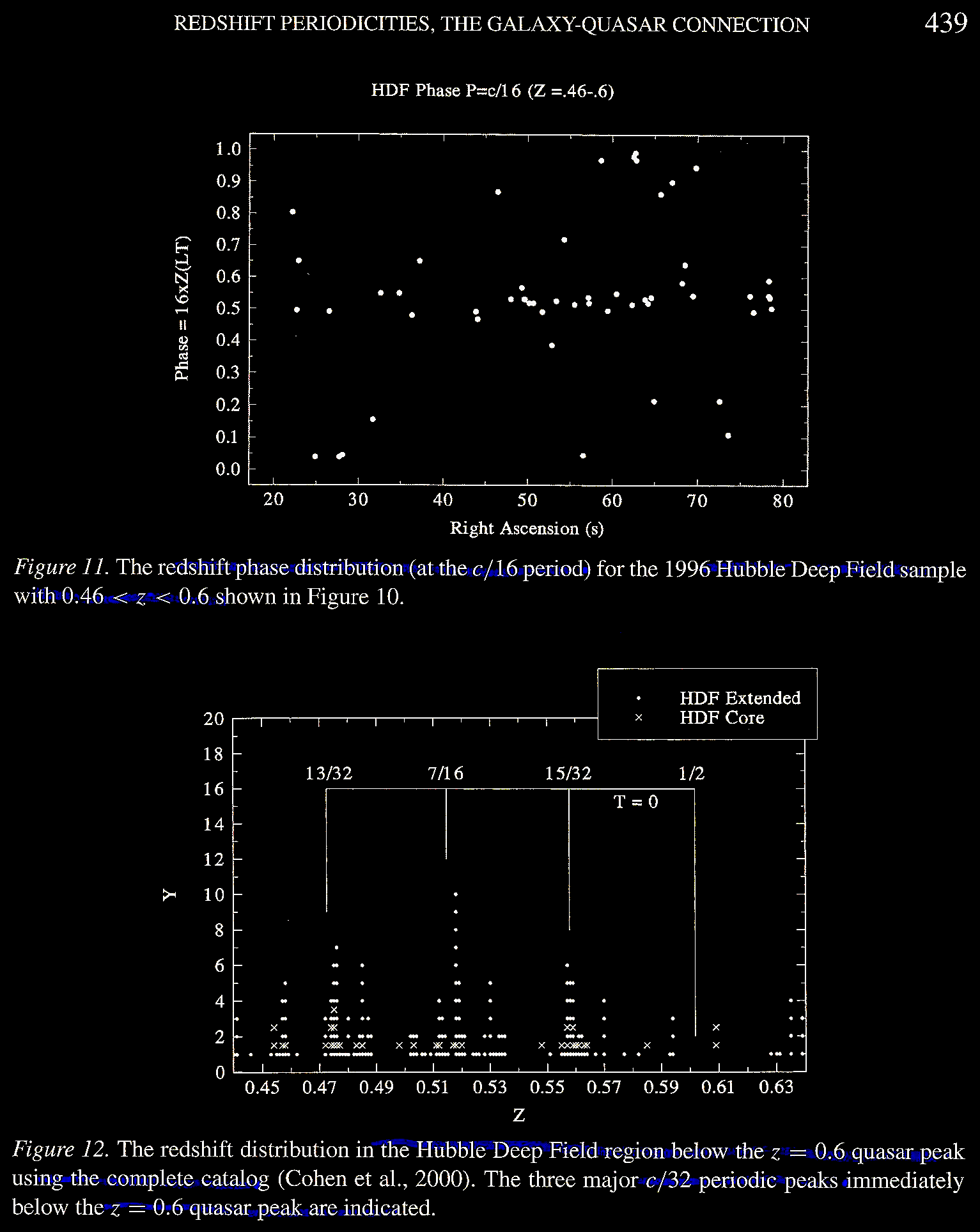
Tifft (2003) Figure 13 shows the
main peaks as well as some "satellite peaks
... offset slightly" from the predicted c/32
and c/16 peaks. Note that all of the
fractions are odd (not even) fractions.
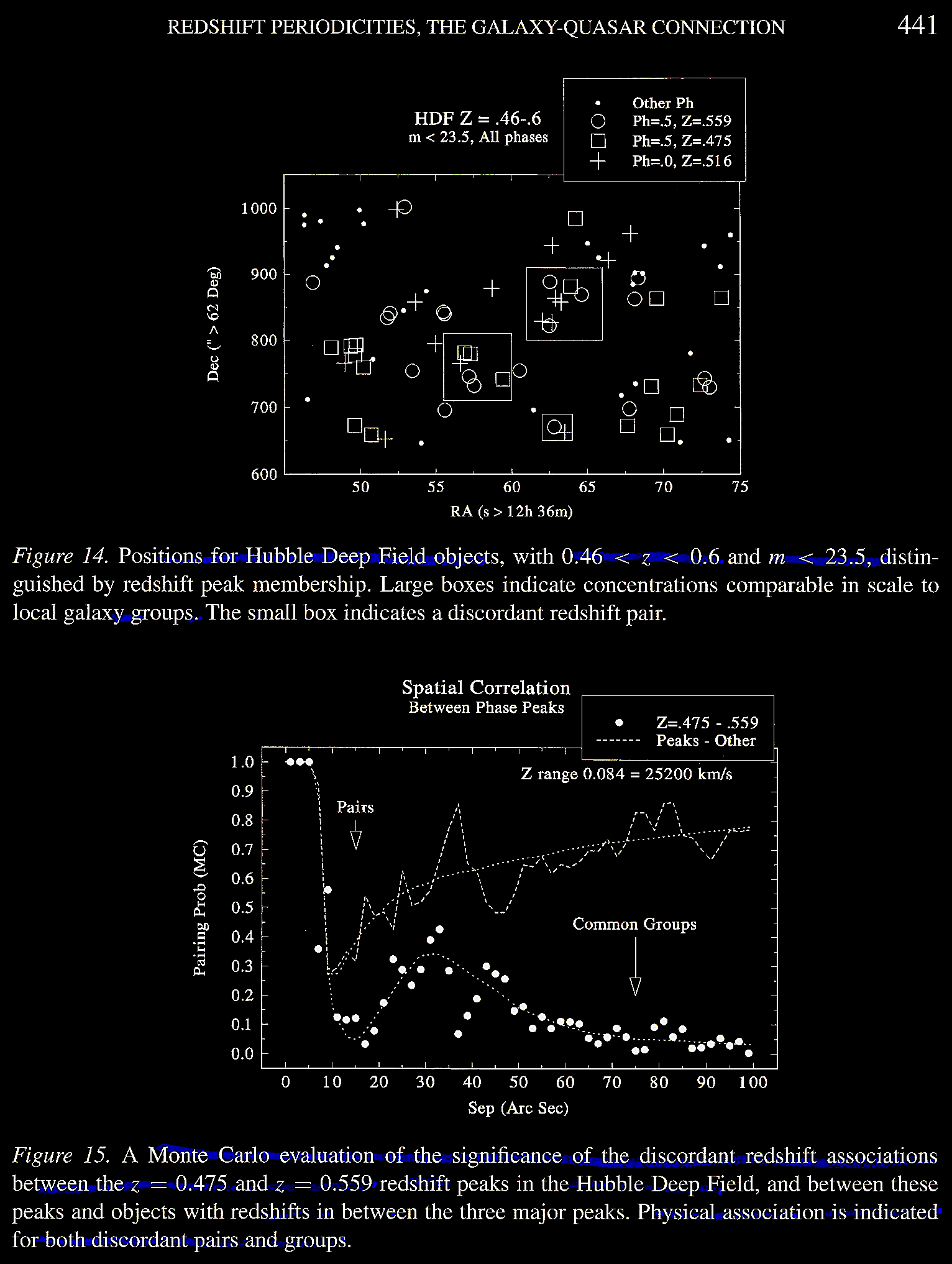
In Tifft (2003) Figure 14, we find
the sky positions of the "extended study"
region of the HDF within certain z
and magnitude (m) values,
designations of galaxy clusters (~1 Mpc),
and also marking of the discordant redshift
pairs of galaxies. Figure 15 shows where
Tifft (2003) asked D. Christein Monte Carlo
statistical analysis of the probability of
pair association by "angular separation"
distribution between pairs of sources with
discordant redshifts compared with 1000
random sample displacements (in RA and Dec)
of objects in one z peak compared
with another. Figure 15 also shows the
difference between two peaks separated to
the extreme by redshift values equivalent to
25,000 km s–1, showing evidence
of clear physical association.
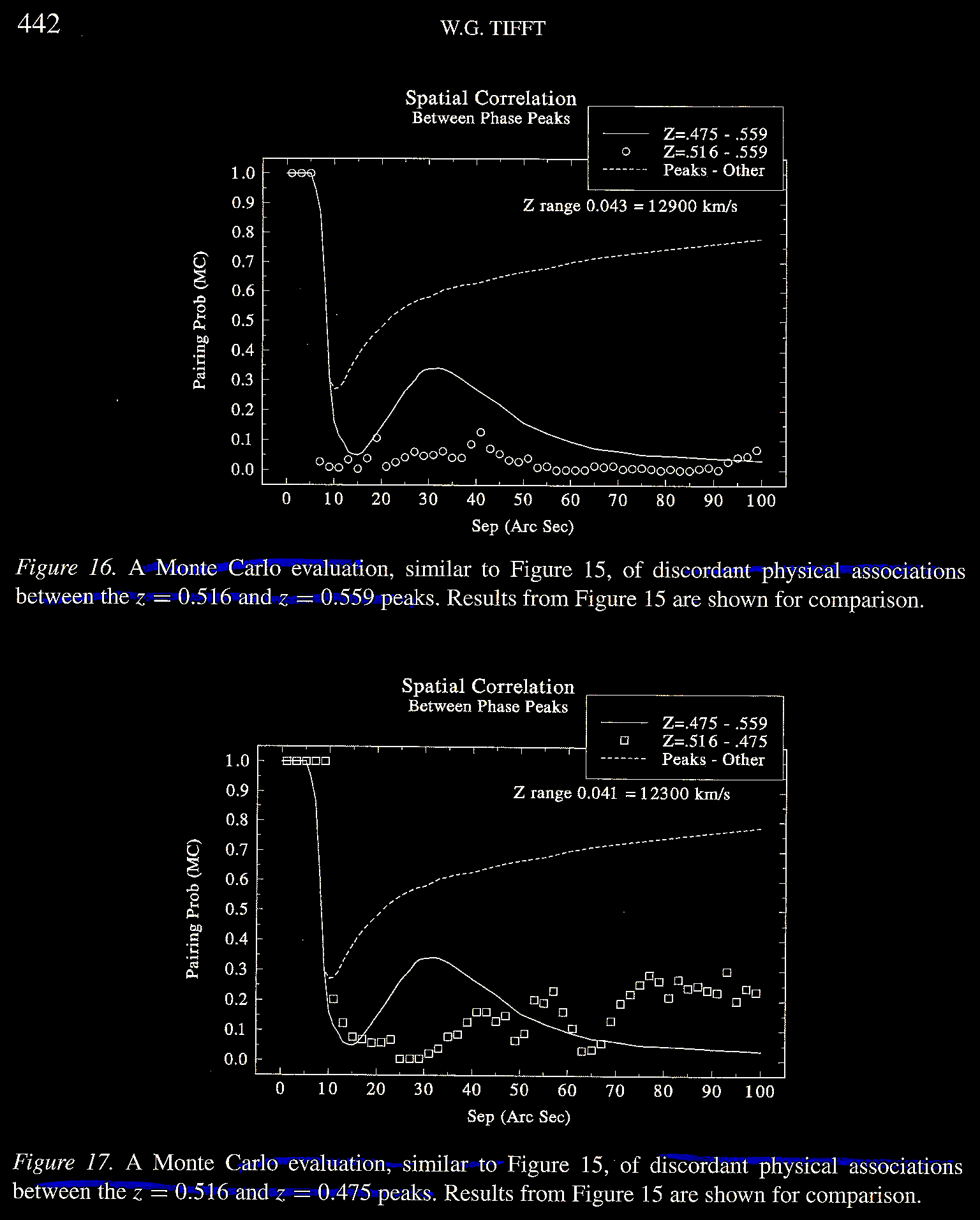
Tifft's (2003) Figures 16 and 17
show the Monte Carlo association analysis
for adjacent peaks with discordant redshift
differences equivalent to the moderate
12,000-13,000 km s–1
range.
Just as they had done HDF
extensions into the higher redshift values,
Tifft (2003) extended the search for
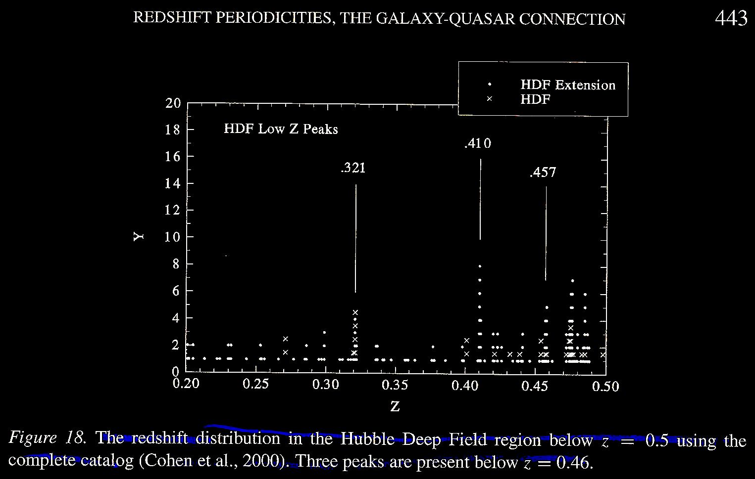
redshift peaks into the lower redshift
values in Figure 18.
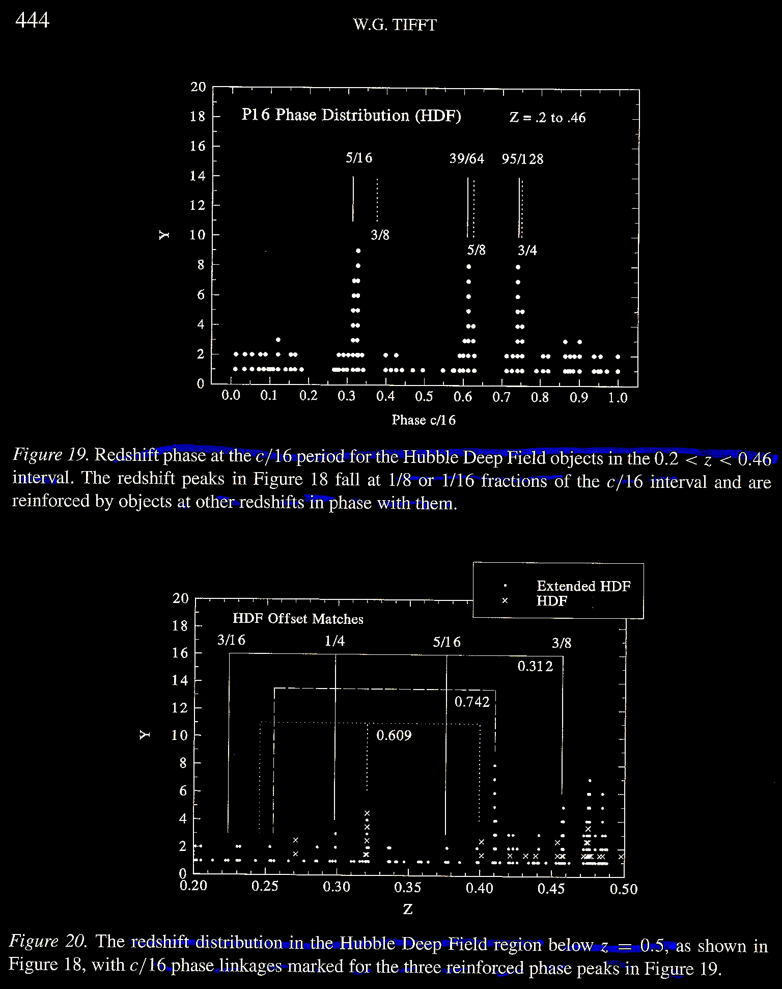
Just as satellite 'phase' peaks
have been observed around certain values in
the HDF, Tifft (2003) Figure 19 shows
'phase' peaks around the value c/16
for the data range of 0.2 < z
< 0.46. Figure 20 shows 'phase' or
satellite peaks around c/16 for z
< 0.5.
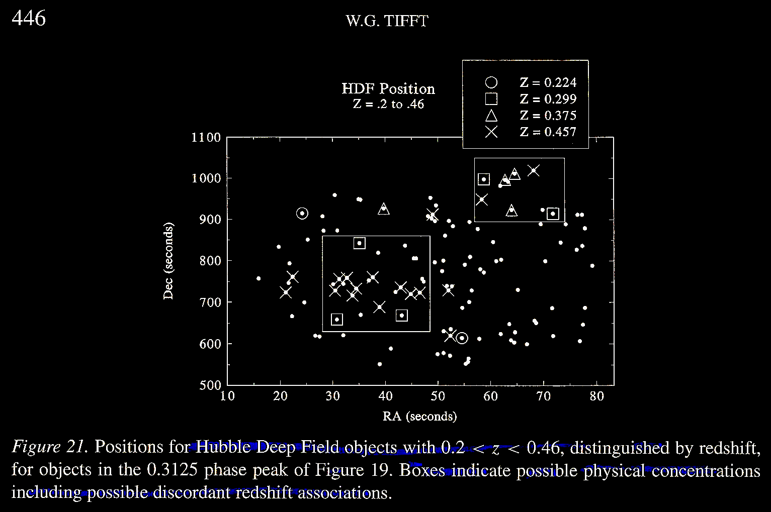
The last step in
analyzing the lower redshift cohort for Tifft (2003) was to
locate their positions on the celestial sphere in RA and Dec
(Figure 21), in order to assess which 'clumpings' may
represent physical associations between sources with
discordant redshifts. Again, there are suggested physical
associations of galaxies with discordant redshifts.
In 1998, another deep exposure was
taken with the HST called the Hubble Deep
Field South (HDFS; https://stsci-opo.org/STScI
from https://hubblesite.org/contents/media/images/1998/).
Cf. full
story link. Even under the ideal
Earth-based conditions at the Cerro-Telolo
Inter American Observatory, this is the
Earth-bound view of the HDFS region of the
sky:
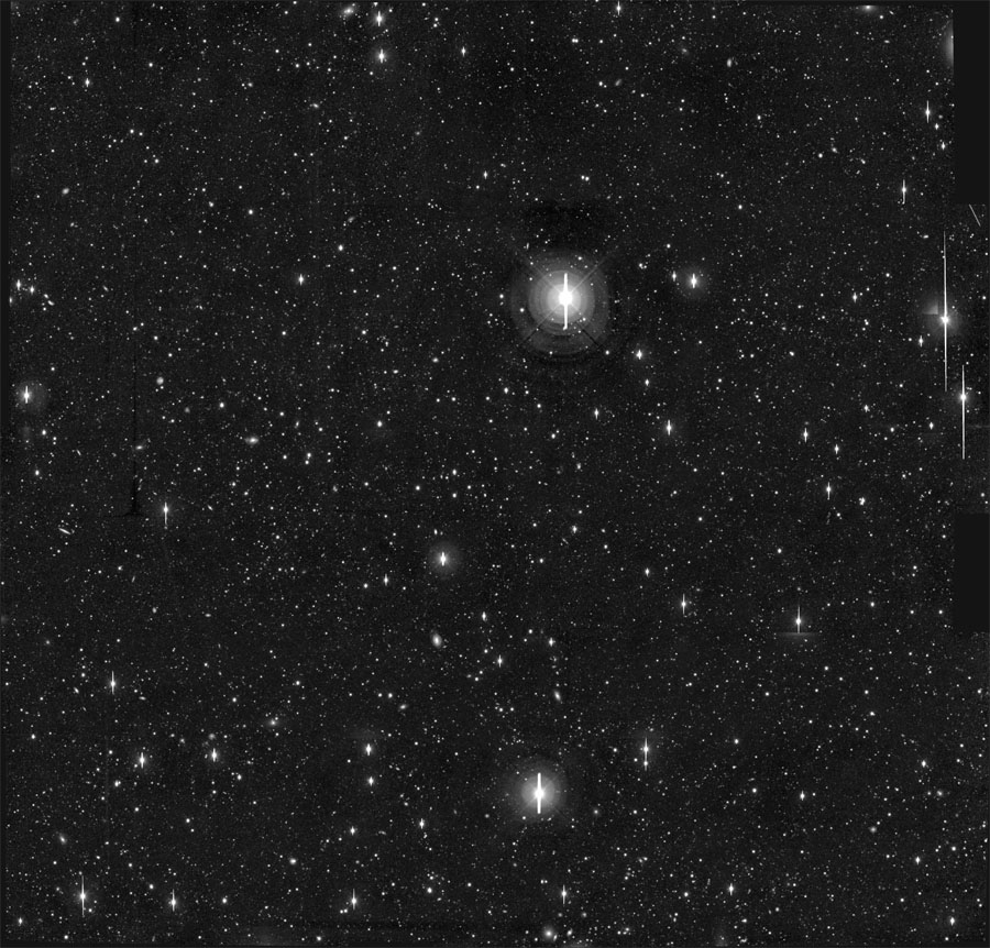
Credit: J. Gardner (NOAO/GSFC), Cerro Tololo Inter- American Observatory (https://hubblesite.org/contents/media/images/1998/).
_23nov1998.jpg)
The HDF findings were tested on
the HDFS. It is no surprise that such
periodicities were found there as well in
the opposite celestial hemisphere. Tifft
(2003) Figure 22 shows sources with
redshifts from 0.3 < z < 0.6,
and sure enough, there are stark
periodicities in the predicted T = 0
around c/64 and c/32, as
well as some peaking associated with the T
= 6 state.
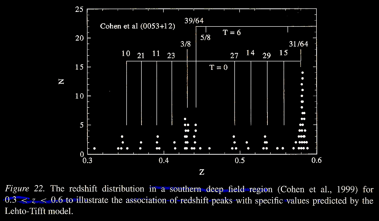
Tifft (2003)'s Figure 23 shows the
'phase' peaking around the c/32
periodicity in the HDFS.
Summary on the Lehto-Tifft
model. The Tifft (2003) study was
presented at a conference of friends,
colleagues, and some old rivals honoring the
widely-loved and admired, great astronomer
and cosmologist Sir Fred Hoyle and the quest
to "better understand the cosmos that Fred
so loved." Sir Fred would have much enjoyed
the presentation, pouring over the data, and
a bracing discussion. While the Lehto-Tifft
model shows a striking agreement of
numerical results with a model of redshift
periodicity built up from the use of a
double decay process from the Planck state,
it still is a pattern-fitting empirical
model, which only hints at the processes
underneath. We note the importance of the
model of these astounding data which are so
unexplained in standard HBB cosmology, and
as the literature cited above references,
mainstream cosmologists have tended to
dismiss or pretend that the redshift
periodicities are not real phenomena. In
what follows, we will explore a little more
data bringing us up to more contemporary
times, and some other possible cosmological
models to explain these data. (Other reading
and resources can be found at link
& link).
Return
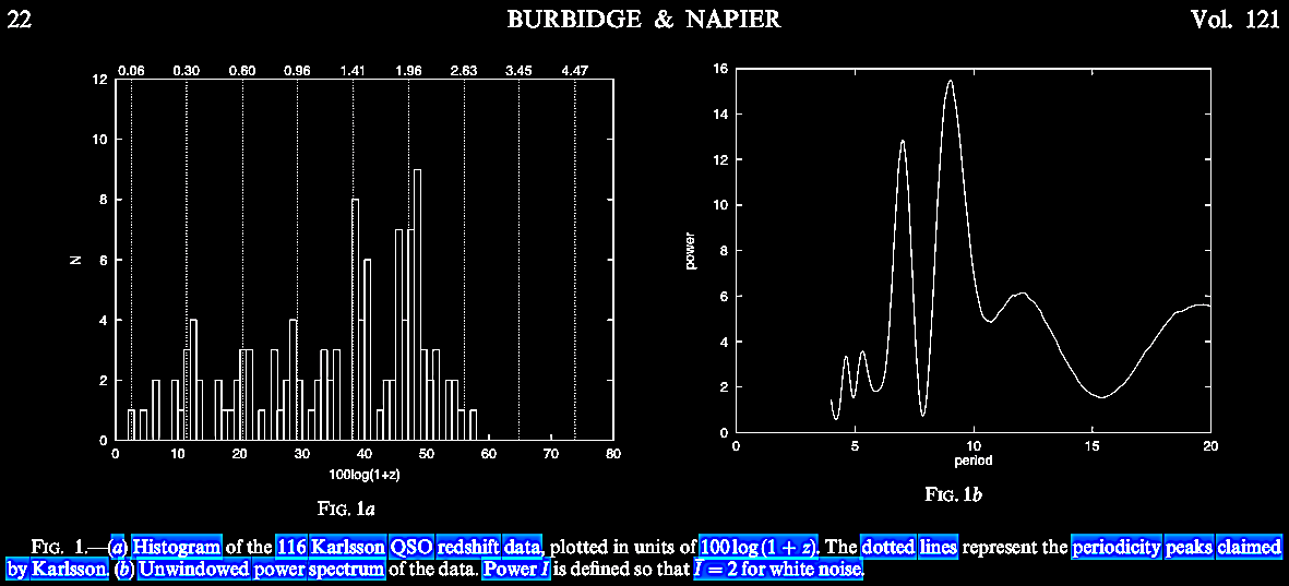
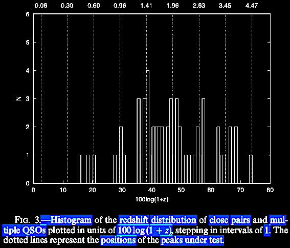
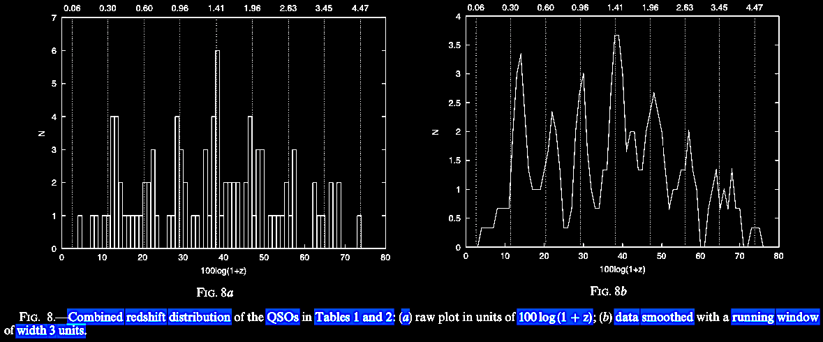
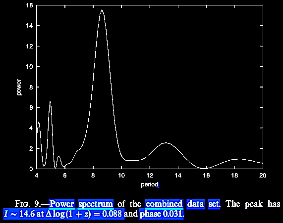
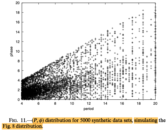
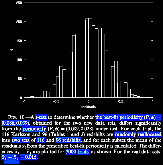
to the Karlsson periodicity. We return to the Burbidge
& Napier (2001) paper. Ever since 2001 with more
complete sets of quasar data, Burbidge, G. & Napier, W.
M. [2001. The distribution of redshifts in new samples of
Quasi-stellar Objects. AJ 121 (1), 21. https://doi.org/10.1086/318018]
found direct observational evidence for the next set of
predicted by the Karlsson formula of redshift periodicity
peaks, z = 2.63, 3.45, and 4.47, beyond what had
been empirically observed up to then. In careful fashion,
Burbidge & Napier (consulting with Margaret Burbidge and
Sir Fred Hoyle) not only ran statistical tests but laid out
the possible interpretations or hypotheses to explain these
data.
 |
 |
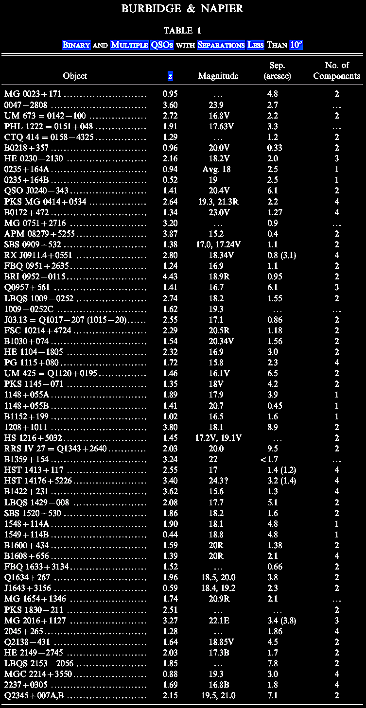  |
   |
  |
 |
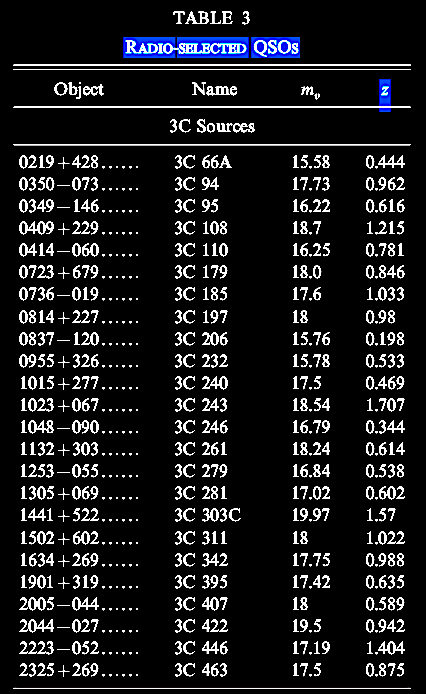 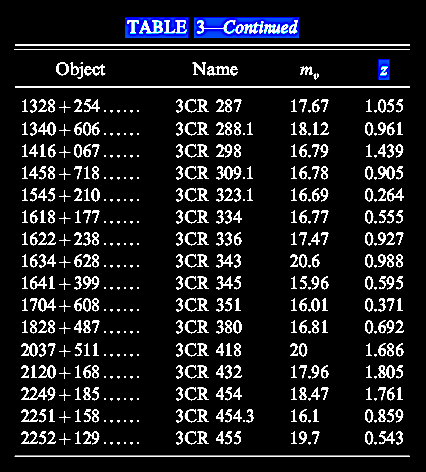 |
Table 3
continuing with 3C radio sources: z-values in
the 4th column: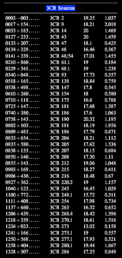 |
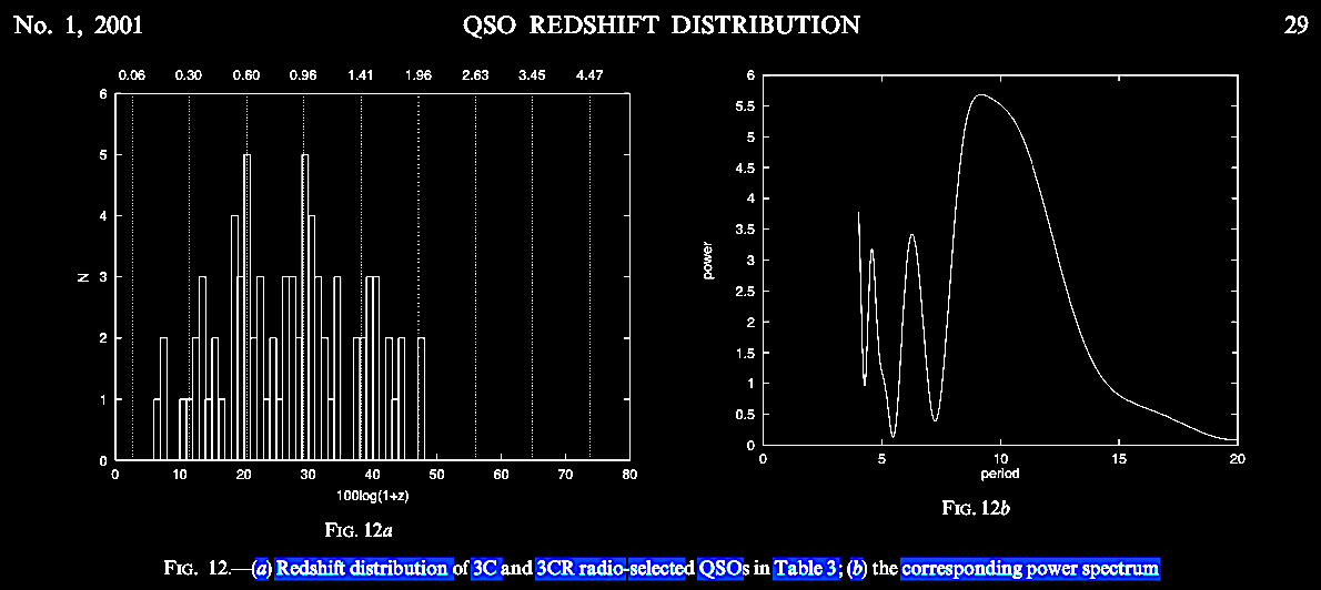
With the QSO data
available in 2001, the Karlsson periodicity continued to
appear and extend beyond and confirming previous predictions.
In 2009, Burbidge
& Napier published another paper, Associations of
high-redshift Quasi-Stellar Objects with active, low-redshift
spiral galaxies. ApJ 706 (1), 657. https://iopscience.iop.org/article/10.1088/0004-637X/706/1/657,
where they were able to affirm that the statistically-robust
associations between higher redshift quasars and lower
redshift galaxies in earlier data sets remained, but were
unable to reproduce the results with a partial data set from
the SDSS at that point. The observations suggesting
associations between low redshift active galaxies and higher
redshift continued to build on the trend since the 1950s and
1960s, where the Ambartsumian-Vorontsov-Vel'yaminov-Arp (AVVA)
ejection cosmogony of galaxies recommends itself as a model
(see the discussion in chapter IX. Vast jets and galactic ejection
phenomena: Mass origin-ejection?).
A
year before the courageous and persistent dissident
observational astronomer Halton Arp's death, more results
were published on the 2dF survey in Fulton, C. C. & Arp,
H. C. 2012. The 2df Redshift Survey. I. Physical association
and periodicity in quasar families. ApJ 754
(2), 134. https://doi.org/10.1088/0004-637X/754/2/134.
(Some of the curated data has been placed at http://casjobs.sdss.org/CasJobs/
and http://tdc-www.cfa.harvard.edu/2mrs/2mrs_v240.tgz).
They examined data from the 2dF Galaxy Redshift Survey
(2dFGRS) and from the 2dF Quasar Redshift Survey (2QZ) in
the two declination strips at Dec 0o and -30o.
In order to avoid a range of mixed redshifts of galaxies and
quasars, they filtered out all but quasars z
≥ 0.5. Making no mention of the Lehto-Tifft model, Fulton
& Arp searched for Karlsson-type periodicity in quasar
redshifts. Around each galaxy, they detected quasars which
conform to "empirically derived constraints based on an
ejection hypothesis." They "ran Monte Carlo control trials
against the pure physical associations by replacing the
actual redshifts of the candidate companion quasars with
quasar redshifts drawn randomly from each respective ...
[R.A.] hour." When properly constrained for quasar z
grouping and the Karlsson periodicity, the 2dF data showed
that the Karlsson periodicity is statistically significant,
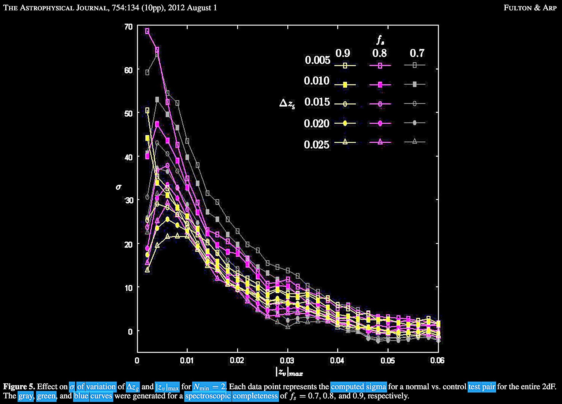
and not a selection effect (Fulton & Arp, 2012; Figure
5).
Fulton
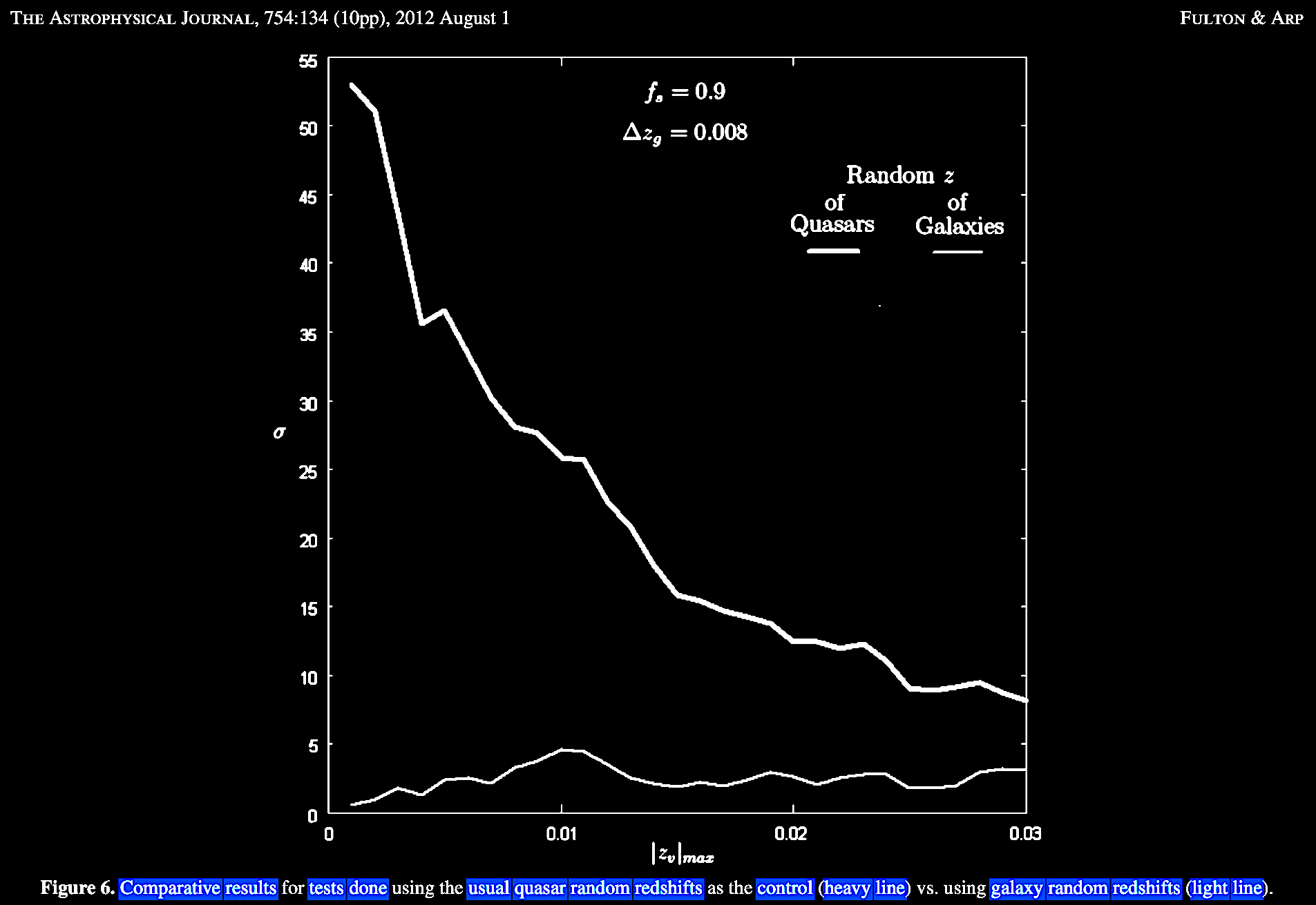
& Arp (2012) Figure 6 shows that the presence of
discordant redshift data between physically connected
galaxies and quasars has been shown to be statistically
significantly.
One
of the more recent papers which has attempted to pull
together the data on redshift periodicity and compare
theoretic explanations was first submitted for publication
in 2016, but only published in 2020, indicating the ongoing
difficulty of suggesting alternative hypotheses for unusual
phenomena in cosmology, and getting them published. That
paper is from an Indian group, Mal et al. 2020.
Periodicity of quasar and galaxy redshift. Astron &
Astroph. 643, A160. https://doi.org/10.1051/0004-6361/201630164.
They briefly and informally review >5 decades of
published research on periodic redshift data. As already
noted, there have been empirical / numerical formulations of
the periodicities observed. And there've been attempts, as
seen above, to model the causes of the observed
periodicities. For example, Depaquit, S., Pecker, J. C.
& Vigier, J. P. 1985. Astron. Nachr. 306
(1), 7. https://adsabs.harvard.edu/full/1985AN,
argued that the periodicities were caused by (1) a selection
effect from data sampling; (2) the non-randomness of quasar
distribution in the Universe, and (3) the presence of
Dopplerian / non-Dopplerian contributions to redshift. Lehto
(1990. Chin. J. Phys. 28, 215) and Tifft
(1997; 2003) proposed their developed explanation, discussed
above.
In
2007, Bajan & Flin published a review called, Redshift
periodicity. Old New Concepts Phys. IV, 159.
http://merlin.phys.uni.lodz.pl/concepts/2007_2/2007_2_159.pdf,
in which they reviewed studies published since the late
1960s up to their date on the redshift periodicity issue. In
their review they included the famous periodicity paper
published by K. G. Karlsson (1971. Possible
discretization of quasar redshifts. Astron.
Astrophys. 13, 333. https://adsabs.harvard.edu/pdf/1971)
who found peaks empirically predicted in a geometric series:
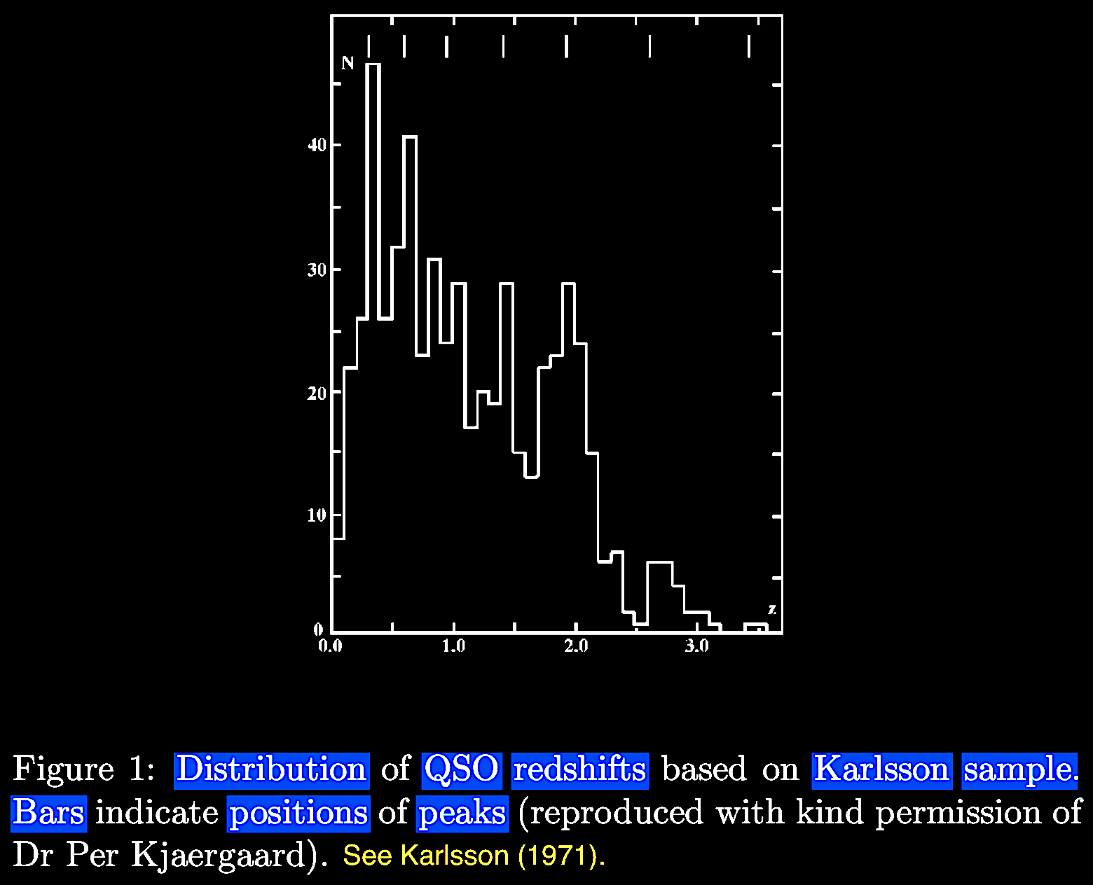
z = 0.3, 0.6, 0.96, 1.41, 1.96, and predicted at 2.63
and 3.46 (Bajan & Flin, 2007; Figure 1), as well as the
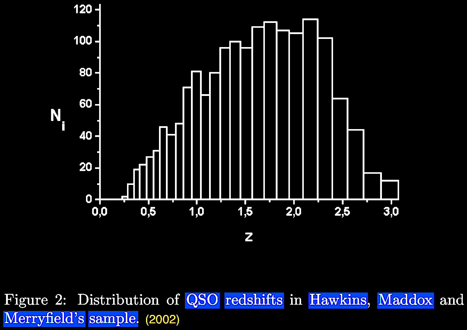
extensive analysis of Hawkins E., Maddox S. J., &
Merrifield M. R. 2002. MNRAS 336 (1), L13.
No periodicities in 2dF Redshift Survey data. https://doi.org/10.1046/j.1365-8711.2002.05940.x.
(Bajan & Flin, 2007; Figure 2), from the SDSS data set.
 |
 |
Many years earlier, following in the empirical astronomy trail-blazed path of Viktor Ambartsumian (1954, 1958, 1961, cf. Arp, 1999. Ambartsumian's greatest insight - the origin of galaxies, in Terzian, Y., Weedman, D., Khachikian, E., [eds.], Active Galactic Nuclei and Related Phenomena, IAU Symposium 194, 473; where Arp recounts Jan Oort's privately whispered confession to him in 1973 that 'You know, Ambartsumian was right about absolutely everything'), Narlikar, J. V. & Das, P. K. 1980. Anomalous redshifts of quasi-stellar objects. ApJ 240, 401. https://articles.adsabs.harvard.edu/full/1980ApJ; and Narlikar, J. V. & Arp, H. 1993. ApJ 405 (1), 51. https://adsabs.harvard.edu/full/1993ApJ argue that QSO redshift periodicities are the result of active galactic nuclei (AGN) ejecting quasars, in accord with the even earlier proposal of a conformally-invariant Machian 'variable mass hypothesis' of Hoyle, F. & Narlikar, J. V. 1964f. A new theory of gravitation. Proceedings of the Royal Society of London. Series A. Mathematical and Physical Sciences 282, 191. http://dx.doi.org/10.1098/rspa.1964.0227; and 1966. A conformal theory of gravitation. Proc. Royal Soc. London 294 (1437), 138. http://dx.doi.org/10.1098/rspa.1966.0199) developed in the elaborations of the CSSC, post-1948; in their C-field formulations).
Theoretical models aside momentarily, the trail blazed by Viktor Ambartsumian and later championed by Halton Arp in galactic cosmology, we in this history tentatively call the Ambartsumian-Vorontsov-Vel'yaminov-Arp (AVVA) cosmogony. Next we turn aside briefly to an excursus on a Machian accounting for anomalous, discrepant or discordant redshifts and redshift periodicity.
References below are cited in full in the Select Bibliography & Resources in the home page).
| In 2017, Narlikar and colleagues published
again on the redshift periodicity problem applying the
HN Machian theory within a larger collection of essays
in honor of Halton Arp (1927-2013): Narlikar, J. V.,
Vishwakarma, R. G., Banerjee, S. K., Das, P. K., &
Fulton, C. C. 2017. An empirical approach to periodic
redshifts. In Fulton, C. C. & Kokus, M.
(eds.). The Galileo of Palomar: Essays in Memory
of Halton Arp. Montreal, Canada: Apeiron; pp.
341-358. http://haltonarp.com/inc/memorial/TheGalileoOfPalomar.pdf. When QSOs were discovered in 1963, their super high redshifts could either be (a) Doppler shifts, (b) gravitational redshifts, or (c) cosmological redshifts, which is due to the 'expansion' of the Universe, the Hubble-Lemaître law, which was quickly the standard view. If the latter or (c) is true, the QSO redshifts should distribute as (eq 1) z = F(r), where z is the redshift, r is the distance, and the function F(r) would tend toward H0 r/c with H0 being the Hubble's constant and c the velocity of light. Under a simple cosmological Hubble-Lemaître interpretation, the probability of the angular distribution and separation between any distant quasar (Q) and any angularly-juxtaposed foreground galaxy (G) should be (eq 2) p = π.∆2n, where the likelihood of chance near juxtaposition, p should be a small fraction of unity, say p ~ 10−4, consistent with the Hubble-Lemaître law. However, if the near angularly-juxtaposed redshifts zG and zQ are different, then there's an anomalous discrepancy with the Hubble-Lemaître interpretation in those cases. Furthermore, if there are evidences of tidal interaction between or even more 'on the nose' a jet connecting the objects with discrepant redshifts zG and zQ, then we have a class of interacting objects which contradict the Hubble-Lemaître law. Over the years and now decades, the data for anomalous galactic redshifts now includes not only objects in the optical wavelengths, but also in the radio, x-ray, and gamma ray wavelengths. Furthermore, the range of known anomalous z-values has not expanded in a smooth distribution but are clustered as discussed around discrete values such that for small z, there is an arithmetic progression (Tifft, 1976) and a geometric progression of (1 + z) for larger z-values (Karlsson, 1977). These discrete or periodic values may be designated (Z1, Z2, ... , ZN), where (eq 3) (1 + ZN) = λN × (1 + Z0), where λ ~ 1.228, and Z0 = 0.06, &c. The Hubble-Lemaître law cannot explain such a effect. This persisting problem has been by most cosmologists ignored for the following pretexts (or excuses, if you will). These stubbornly anomalous data....
So starting with the Hubble-Lemaître flow, there seems to be an excess 'intrinsic' component in systems where any QSO Q with redshift zQ is in apparent physical association with a galaxy G with redshift zG. Applying the Ambartsumian-Vorontsov-Vel'yaminov-Arp (AVVA) cosmogony as a working hypothesis, where higher redshift QSOs originate and are ejected from active galactic nuclei (AGNs) with an intrinsic redshift component, such that zQ >> zG in general and the intrinsic component, zI, is defined in empirical terms with the equation: (1 + zQ)
= (1 + zG)(1 + zI)
(4)
Narlikar and colleagues now proceed to lay out an alternative theoretic framework to explain these data, in terms of the AVVA cosmogony. The underlying mechanism was proposed during a fruitful period as the Machian theory of gravity by Hoyle & Narlikar (1964f, 1966d) in the C-field context of the Classic Steady State Cosmologies (CSSC). {It is important to note that Stephen Hawking's (1965) famous claim during the HBBC-CSSC controversy about falsifying infinities in the HN theory has long been falsified: See below: Appended Note on Replies to Hawking, 1965}. Narlikar adapted the HN Machian theory to explain the anomalous redshifts within the AVVA cosmogony context thus (cf. Narlikar, 1977; Narlikar & Das, 1980, cf. 1975; Narlikar & Arp, 1993, 1997) and the dynamics of ejection in Narlikar et al. (2002): The field equations of the Hoyle-Narlikar theory are [eq dim: w = 377 and 392 in honor of Narlikar & Hoyle respectively by date] 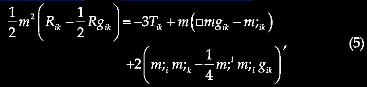  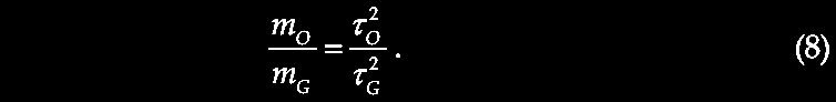 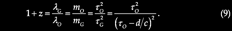 Expanding universe case. Now, moving to the 'expanding universe' case, as Hoyle & Narlikar (1971) argued, this VMH redshift is precisely what one gets in an 'expanding cosmos' with particle masses, m1, m2, ... , mN, remaining constant. However, since the Hoyle-Narlikar theory is conformally invariant (unlike general relativity), standard relativistic cosmology can be obtained from (6) the simplest line element in Minkowski spacetime by this conformal transformation   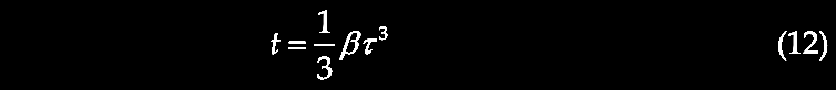  And then t-time in the traditional line element is simply the standard cosmic time of Friedmann (HBBC) cosmology and the redshift formula gives the same expected result as (9) above. The Friedmann cosmology by insisting that particle masses at all epochs are constant (a) forces spacetime to be non-Euclidean (contrary to observational data), (b) leads to a spacetime singularity (classic Big Bang) / singularities (black holes), and (c) exiles the never-vanishing question of matter creation (non-conservation of baryon number) back to some singular, energetic unification epoch post-t = 0. As Khembavi (1978) showed in his 'Zero mass surfaces and cosmological singularities' study, under general conditions, the zero mass 3-hypersurface at t = 0 forms a singularity under the conformal transformation Ω ∝ m and all the singularities under the singularity theorems expected by Penrose (1965), Hawking & Ellis (1973), and Hawking (1977) are found and explained. As Khembavi notes, contrary to Hawking & Ellis (1973; p. 364) and Hawking (1977), the presence of singularities in general relativity is no virtue, and contrary to the rest of physics—recognizing that conformal invariance is a symmetry of Nature (as Khembavi points out). Within the Hoyle-Narlikar conformally invariant theory, Khembavi showed, there are a number of non-singular cosmological models possible (citing also the Hoyle & Narlikar, 1974 opus). The Hoyle-Narlikar Machian-based flat cosmology described can be augmented so that rather than assuming that all matter originates at some τ = 0, we allow that matter can also originate repeatedly and episodically wherever and whenever the energetic conditions in the AGN of galaxies reach thresholds to manifest as the creation and ejection of compact objects like QSOs (as in the AVVA cosmogony). So, in the AGN of the galaxy (G), the particles of the new QSO are similar but start with a zero mass 3-hypersurface at τQ, gaining mass by Machian interaction with a growing region of the Universe. The formal mathematics and physics of this proposed process is discussed in Narlikar (1977), building on earlier work done by Hoyle and Narlikar in the 1960s. Consider, argued Narlikar (1977), that a conformal theory of gravity (e.g., Hoyle-Narlikar, 1964f; 1966d; 1971), modeled similar to action-at-a-distance electrodynamics (cf. Wheeler & Feynman, 1945; 1949), a series of implications may be found. The HN general theory and its applications in the CSSC, QSSC, and possible oscillating cosmologies will be reviewed in Chapters III and XII. In the same volume,
Fulton, C. C. (2017). From Hubble to Arp. In
Fulton, C. C. & Kokus, M. (eds.). The Galileo
of Palomar: Essays in Memory of Halton Arp.
Montreal, Canada: Apeiron; pp. 293-339. http://haltonarp.com/inc/memorial/TheGalileoOfPalomar.pdf,
summarized the implications of the general Narlikar
(1977) model with the Friedmann (1922) model, both
models are special cases of larger theories of
interpretation of the Hubble-Lemaître relation (Fig.
39):
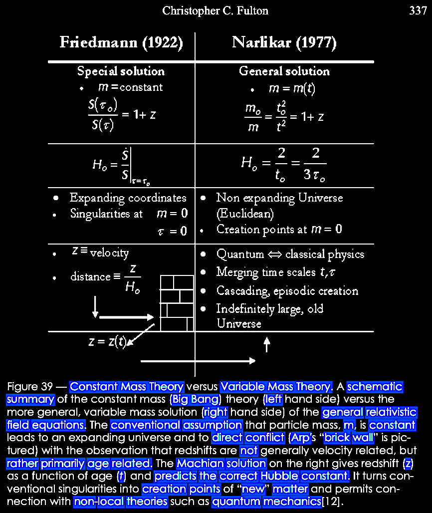 Fulton (2017), Figure 39. The particles in the QSO will grow in mass as    Periodic redshifts. The authors consider the periodic redshift data first in a Minkowski spacetime. Empirically, the authors consider a sample of central galaxies with measured redshifts (zG) with the measured redshifts of paired quasars (z1, z2) in tabular form (Narlikar et al. 2017; Table 1), which are then corrected to the galaxy redshifts to find the putative intrinsic components by (1 + zQ) = (1 + zi) / (1 + zG); i = 1, 2, ... , which are then compared to the nearest periodic peak identified from the sequence Zn given by the Karlsson (1977) formula: Δlog(1 + Zn) = constant = 0.089, Z0 = 0.06, which generates a sequence of redshift values of n = 0, 1, 2, ... , n; where Zn = 0.06, 0.30, 0.60, 0.96, 1.41, 1.96, 2.64, &c. Arp et al. (1990) have claimed that QSO redshifts seem to be distributed preferentially close to the Karlsson sequence values. 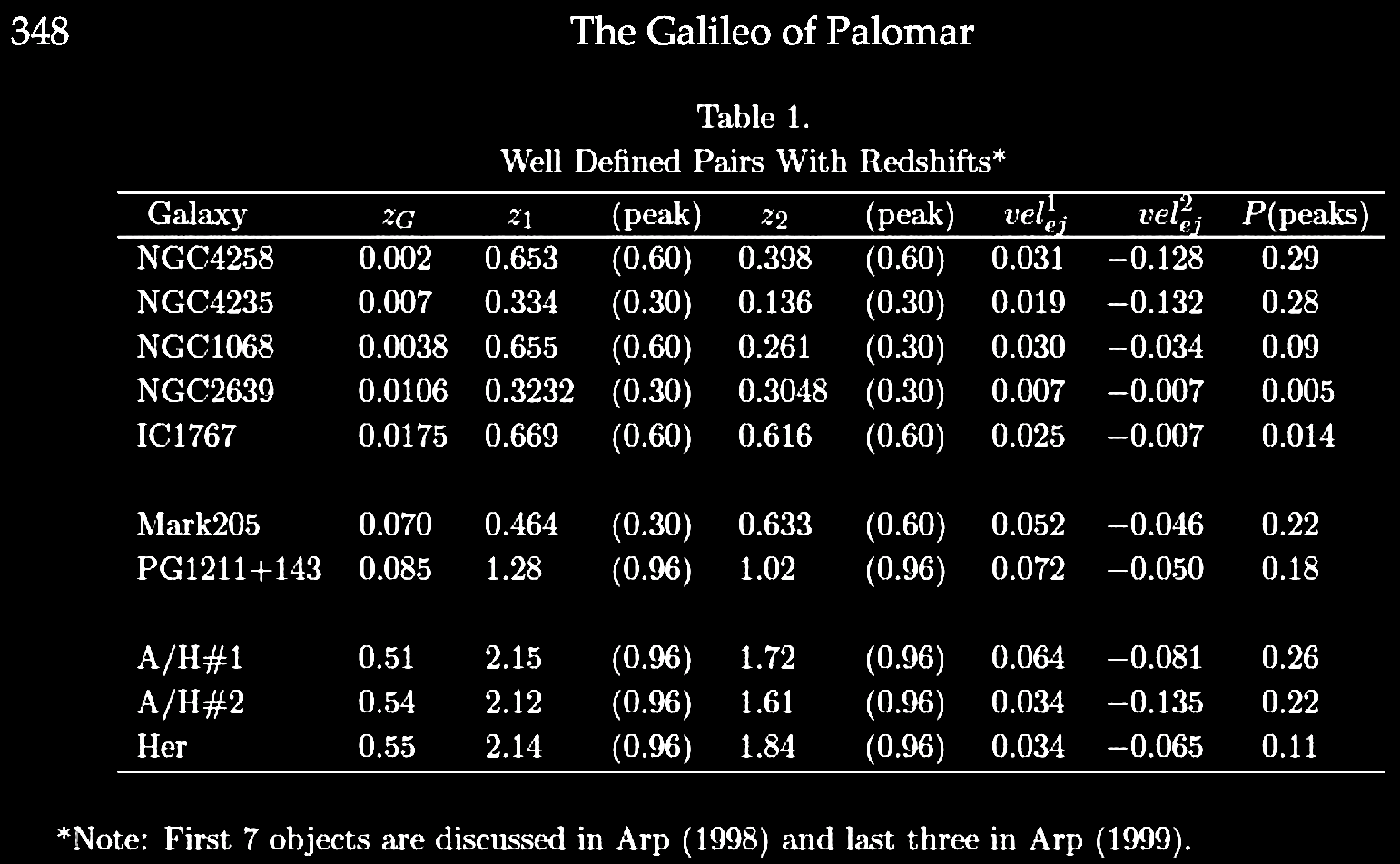 With respect to the data compiled in Table 1, Narlikar et al. (2017) proposed to test the following hypothesis: The differences between zQ and the nearest peaks are postulated to be the true Doppler velocities of ejection as viewed by the observer (O), i.e., (1 + zej) = (1 + zQ) / (1 + Zp), where Zp is nearest Karlsson peak. These calculated values of ejection velej (columns 7 and 8 of Table 1), show approach toward and recession away from the observer (O) respectively. Except for the first two cases, NGC 4258 and 4235 in the table, which are ambiguous with their low redshifts, zQ values associated with the nearest Karlsson peak yield one QSO approach and the other receding away from the observer (O). It is also possible in the case of galaxy NGC 4235 that the low velocity of approach of one of the ejected QSOs at zQ1 = 0.031 compared with the velocity of recession of zQ2 = −0.128, because it has encountered some resistance slowing down the velocity of ejection. These preferred peaks in higher redshift quasar families associated with galaxies have been further confirmed by Fulton & Arp (2012) in the 2df data, and have since 2017 been again even further confirmed by Fulton, Arp, & Hartnett (2018) in the SDSS and 2MRS data. Even in the small sample in Table 1, the conformity of the quasar pairs to the Karlsson peaks is impressive, the authors note. The statistical significance of the peaks here may be summarized thus (Arp method): Column 9 contains the 'accidental probability' that both QSO redshifts (zQ) fall close to the proximal Karlsson peak (Zp) in the reference frame of the galaxy (G) calculated by taking the difference between zQ and Zp and then dividing that by 1/2 of the distance to the nearest Karlsson peak: {| zQ | – | Zp |} ÷ 1/2 = P(Zp), where each pair is an independent trial and their combined probability is computed, the pair being normalized to 0.5, yielding the probability P that the real QSO pair redshifts fall as close to the Karlsson peak as they do. For NGC 1068, the QSO1 is 0.030 away from Karlsson peak Z2 = 0.60 in the Karlsson interval (0.60, 0.96), so the probability for it is 0.030/0.18. Similarly for the QSO2, the ejection velocity −0.034 is negative with respect to Karlsson peak 0.30, so the Karlsson interval is (0.06−0.30) and the probability is 0.034 / 0.12. The combined probability is 2 × (0.030 / 0.18) × (0.034 / 0.12) = 0.09. Thus, the combined probability for the first 5 QSO pairs is P = 9 × 10⁻⁶, the combined probability for the last 5 is P = 4 × 10⁻⁴, so that the combined probability of all the pairs in Table 1 being randomly close to the Karlsson peak values is P = 7 × 10⁻⁹. In addition to the periodic intrinsic redshift values, the projected QSO ejection velocities seem well matched in magnitude, even though they might not be because of factors such as (a) initial ejections not being exactly opposite, (b) perturbations or collisions of ejected QSOs modifying their projected velocities, and (c) the speed at which the QSO redshifts transition between Karlsson quantized peak values may catch some quasar z-values between peaks. The projected velocities are graphed in Figure 1, where the intrinsic redshift component declines with increased Machian contact with the rest of the Universe, and also the QSO projected ejection velocities decline as the QSOs separate from the putative parent galaxy. 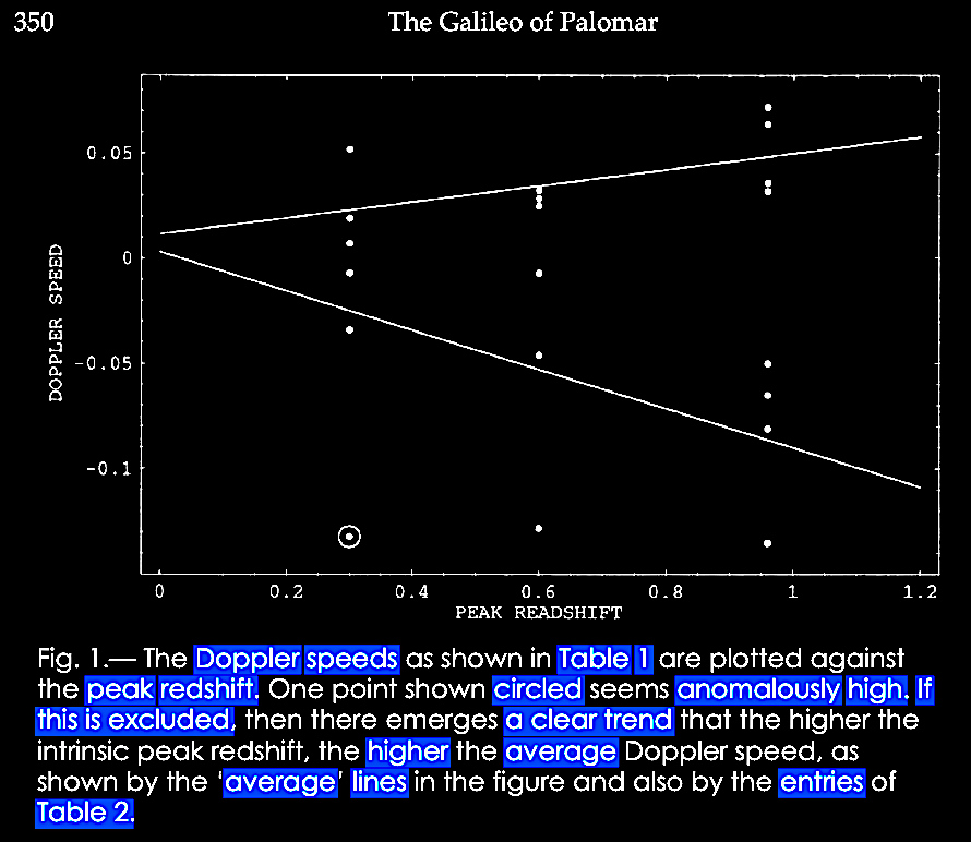 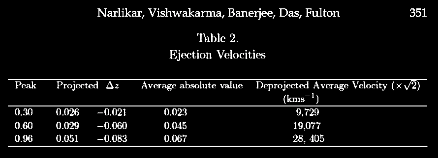 Suppose that the new proto-QSOs are initially held as energetic components in incubative orbits within the active galactic nucleus (AGN), and then later blown out in explosive events at the observed velocities? In the QSSC (Hoyle, Narlikar, & Burbidge, 2000), as in this empirical approach to the VMH, it is argued that creation of matter (baryons) takes place in an increasingly negative energetic region of a negative scalar field (C-field) of Machian origin. As baryon creation proceeds the C-field negative energy builds to a repulsive-explosive threshold overcoming gravity (in the conformally-invariant gravitational field), and the AGN fragments ejecting coherent proto-QSOs, relaxing the C-field energy again below the repulsive-explosive threshold. Assuming that baryogenesis occurs according to the C-field hypothesis and that some as yet unknown quantum process causes the ejection stages, the proto-QSO is explosively expelled from the AGN only exactly when its redshift is at one of the Karlsson peak values. So periodic Karlsson peak-z data require modifying the original Narlikar-Das hypothetical scenario. Using a t coordinate for convenience instead of the τ coordinate, a QSO originating at tQ is bound in incubative orbit in the AGN and not ejected until time tE when the proto-QSO's intrinsic VMH redshift is decreased through Machian interaction to zE—such that the intrinsic VMH redshift zI —> zE, a member of the Karlsson sequence values Zn, and zE determines the time of ejection, tE., as observed in galaxy O when the QSO's light arrives at time tO: 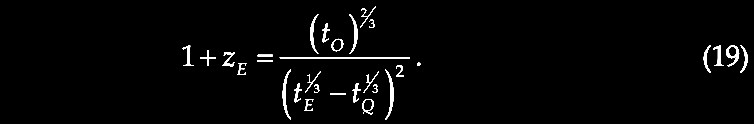 Integration of the equation of motion from Narlikar et al. (2002) yields the velocity ω of the QSO at that point in time. Using a composite redshift formula combining both Doppler effect as well as VMH, observed redshift zQ can be related to speed ω and the angle to the line of sight α in the local spacetime [R, T] coordinates from Narlikar et al. (2002): 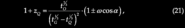
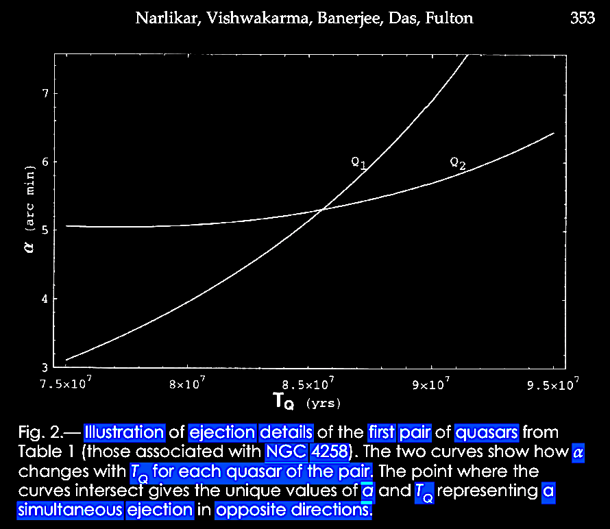 The first three QSO pair cases in Table 1 are analyzed using the above procedure, and the results placed in Table 3, where column 1 has the designation of the galaxy and its redshift, and the rest of the parameters in their respective columns, ending with the nearest Karlsson peak (Zp) in the last column, so that Table 3 may be thought of as the beginning of a more refined version of Table 1, on the dynamics of quasar ejection: 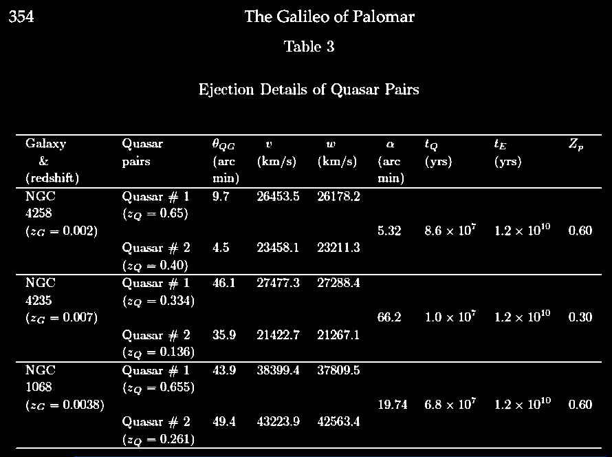
    An underlying quantum theory yet to be discovered? Unlike most authors, these authors take the finding of periodic redshift peaks a series first discovered by Karlsson seriously. Using the VMH, they showed that as a new QSO created in an AGN galaxy, its particle masses increase with time through Machian interactions with the Universe. In a classical VMH, the mass has a steady and continuous decline of the QSO intrinsic redshift from infinity in the beginning at tQ = 0 to finite values at the time of QSO ejection. Using mass × (1 + z) = constant from the modified VMH suggests that particle masses in the new QSOs should exhibit the Karlsson periodicity peaks. However according to the modified VMH, the newly created QSO 'hibernates' or remains in the AGN until the QSO particle masses match some discretized or quantized Karlsson peak value before QSO ejection, thus revealing the intrinsic redshift peaks we observe! Why? Thus they searched for a theory underlying this phenomenon. So they conceived a heuristic quantum mechanical VMH model (they call it a 'toy model') drawing the obvious comparison between the energy levels in the physics of a simple harmonic oscillator and the peak redshift values in the Karlsson series. In this heuristic quantum mechanical VMH, the discrete or quantized sequence values ln(1 +Zn) forms this arithmetic series:     
 Gamov (1966),
Figure 12:
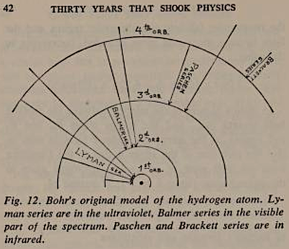 Gamov (1966). The search for that deeper VMH / Machian quantum theory justifying these assumptions and predictions continues. |
Appended Note on Replies to Hawking, 1965: In 1965, Stephen Hawking published, On the Hoyle-Narlikar theory of gravitation. Proc. Royal Soc. A 286, 313. https://doi.org/10.1098/rspa.1965.0146, argued that the Machian HN theory in its time-symmetric retarded and advanced (going backwards in time) relativistic wave equations in integration would diverge to infinity because of the infinite future. Hoyle & Narlikar, in 1995. Cosmology and action at a distance electrodynamics. Rev. Mod. Phys. 61, 113. https://doi.org/10.1103/RevModPhys.67.113, pointed out that 'no normalization is necessary' in HN gravity because unlike the Friedmann cosmologies, the CSSC and QSSC with C-fields meet the requirements of the Wheeler-Feynman absorber theory of radiation in the past light-cones of the Universe as well as in the asymptotic future. Further, as H. Fearn (2015) has shown in Mach's Principle, action at a distance, and cosmology. Journal of Modern Physics 2015 (6), 260. http://dx.doi.org/10.4236/jmp.2015.63031; http://www.scirp.org/journal/jmp, because of the Cosmic Event Horizon (CEH, i.e., observer's horizon) in an expanding, accelerating Universe (as predicted by the CSSC), the advanced solutions indeed would not diverge to infinity given the CEH boundary, and hence, Hawking's objection is mistaken. That an ongoing, robust theoretic development can take place along the conformally invariant HN theoretic lines, is evident in Yadav et al. 2016. C-field cosmological models: revisited. Research in Astronomy and Astrophysics 16 (12), 188. https://iopscience.iop.org/article/10.1088/1674-4527/16/12/188, and in Narlikar (2021), Three pathbreaking papers of 1966 revisited: their relevance to certain aspects of cosmological creation today. EPJ H 46, 21. https://doi.org/10.1140/epjh/s13129-021-00025-6. We will return to this arena further in later chapters. |
Histograms of the periodicities they detected in the SDSS quasar and galaxy redshift data versus the periodicities detected in the mock data, Mal et al. (2020)'s Figures 7 & 8, and Table 3, respectively.
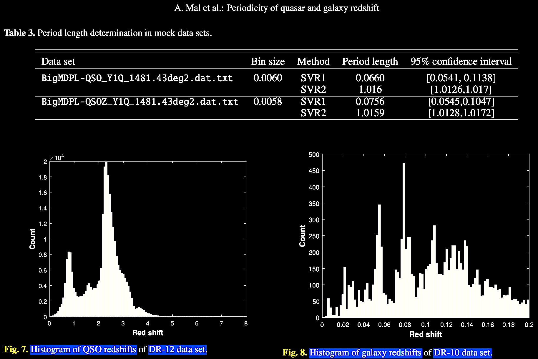
SVR spectra of
redshift periodicities for QSOs and galaxies in the SDSS
data in Mal et al. (2020) Figures 9 and 10.
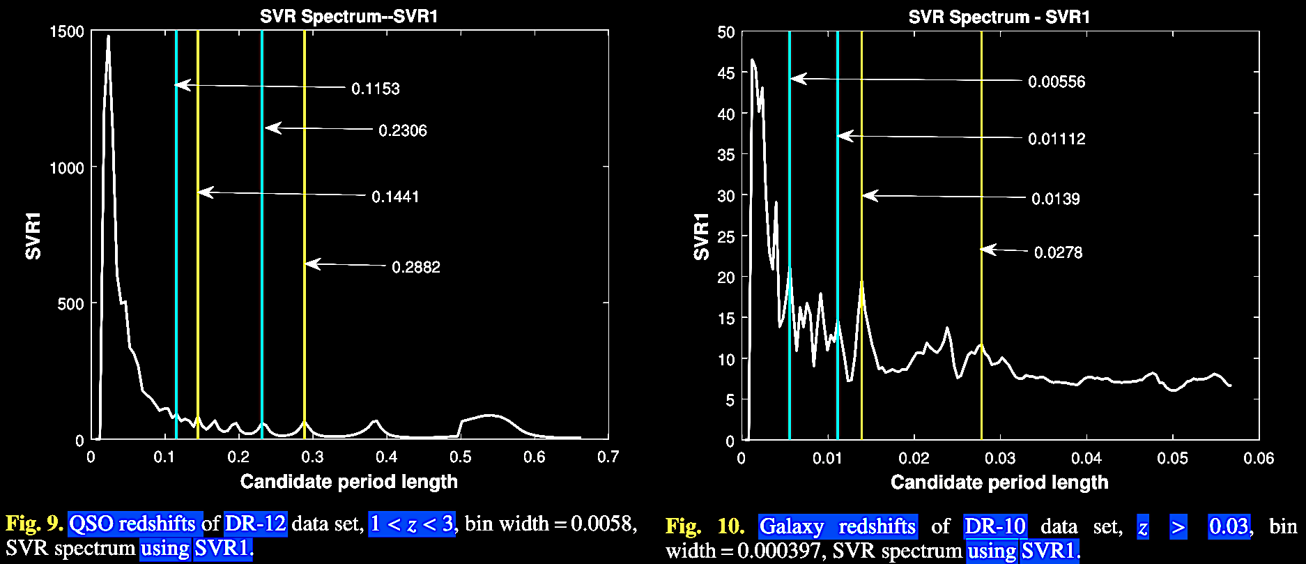
Although it took 4 years to get their paper published, Mal et al. (2020), having reviewed the field of redshift periodicities, made some conclusions on how various theoretical models help explain these phenomena. In the standard HBBC theory, where we have an expanding cosmos which is generally isotropic and homogenous, they point out, the distribution of extragalactic redshifts should be approximately aperiodic and continuous. However, as the data show, they are neither. Since redshift periodicity is really there, Mal et al. in their discussion and conclusions turn to three main theoretical solutions to explain these results:
- i. The
Lehto (1990) model, later developed by Tifft
as we saw, can predict the redshift
periodicities, but it's hard to tell how to
square 3-d quantized time with the rest of
physics.
- ii. The
Roberts, M. D. 2002. Astrophys. Space
Sci. 279, 305 model seeks to
explain discrete redshifts by the spherical
integer 1 which is found in both density
perturbations and in the solutions of the
Friedmann-Robertson-Walker (FRW) spacetime
equations, leading him to find these
significant. However, Mal et al.
indicate that certain assumptions need to be
justified before this theoretical approach
can be pursued further.
- iii.
The Hoyle-Narlikar (1964, 1966) Machian
variable mass theory where matter acquires
properties from 'causal'
interaction-at-a-distance with the rest of
the matter in the Universe, thus suggesting
that new galaxies begin at the 0-rest mass
surface in the solutions and then gain mass
in Machian quantization terms, such that the
multi-component periodicities observed can
indeed be predicted by the HN theory (to
which we will return in later chapters).
- iii(a). To iii
of Mal et al. (2020), I'll further add this
thought: Taking the Hoyle-Narlikar Machian
theoretical approach and considering also the
Ambartsumian-Vorontsov-Vel'yaminov-Arp (AVVA)
galactic ejection cosmogony hypothesis (see Chapter IX),
one may be getting closer to a combined
cosmology-cosmogony more conformable to the data of
our Universe. This was the motivation in part behind
Hoyle, Burbidge, and Narlikar's QSSC papers starting
in the early 1990s, but now with JWST and
accumulating data, we may be moving toward a renewed
Machian CSSC on a far grander scale, an indefinitely
vast or eternal, infinite Universe which
"episodically unfolds itself from many points within
itself" (as Halton Arp in 1998; p. 251, speculated),
numerous points in the Universe, like the centers of
active galactic nuclei (AGNs) where perhaps the CSSC
/ HN Machian / QSSC C-field (or the CGC
model's 'recycling') where the energetic conditions
are met. We will return to these issues in
forthcoming chapters IX, X,
and XI.
In later chapters, we'll also discuss how these phenomena and theoretical considerations are beyond the current New Ptolemaic System paradigm of the ΛCDM Concordance cosmology of the HBBC. We also await the development of the emerging CGC model, by friend and colleague Joe Bakhos, who is taking cognisance of this fascinating and deeply significant class of observations of our Universe. See Bakhos, J. 2022. Chasing Oumuamua: An apology for a cyclic gravity and cosmology, consistent with an adaptation of general relativity. https://vixra.org/pdf/2203.0032v4.pdf, and the further postings at The Taurus Report: https://taurusreport.com/ and its Youtube channel).
In light of these anomalous redshift phenomena, we turn to the wise words from late last century of three of the pioneers of dissent in modern cosmology: Sir Fred Hoyle, Geoffrey Burbidge, and Jayant Narlikar.


Geoff Burbidge, Sir Fred Hoyle, Jayant
Narlikar
"[Because it is outside current
theory] most astrophysicists and cosmologists have felt
justified in ignoring the evidence for anomalous redshifts,
the thought being that what is known to be impossible
remains impossible no matter how strong the evidence for it
may be. . . [Our] main purpose . . . [in] the present paper
is to question this mode of thinking" (Hoyle &
Burbidge, 1995).
We will next turn to the phantasmagorical
world of radio astronomy and the part it has played in the
history of the search for a modern scientific cosmology.